I need help on 2 and 3

on question 2 I got the right numbers is just it appears a negative sign and the 3rd question I can't figure out the equation and the one I used it keeps giving me 0 as an answer, please help!

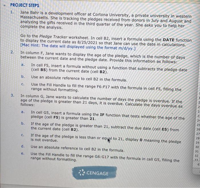
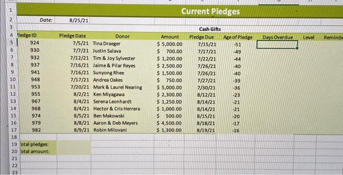
PROJECT STEPS 1. Jane Bahr is a development officer at Cortona University, a private university in western Massachusetts. She is tracking the pledges received from donors in July and August and analyzing the gifts received in the third quarter of the year. She asks you to help, her complete the analysis. Go to the Pledge Tracker worksheet. In cell B2, insert a formula using the DATE function to display the current date as 8/25/2021 so that Jane can use the date in calculations. [Mac Hint: The date will displayed using the format m/d/yy.] 2. In column F, Jane wants to display the age of the pledge, which is the number of days between the current date and the pledge date. Provide this information as follows: a. In cell F5, insert a formula without using a function that subtracts the pledge date (cell B5) from the current date (cell B2). b. Use an absolute reference to cell B2 in the formula. c. Use the Fill Handle to fill the range F6:F17 with the formula in cell F5, filling the range without formatting. 3. In column G, Jane wants to calculate the number of days the pledge is overdue. If the age of the pledge is greater than 21 days, it is overdue. Calculate the days overdue as follows: a. In cell G5, insert a formula using the IF function that tests whether the age of the pledge (cell F5) is greater than 21. b. If the age of the pledge is greater than 21 , subtract the due date (cell E5) from the current date (cell B2). c. If the age of the pledge is less than or equal to 21 , display 0 meaning the pledge is not overdue. d. Use an absolute reference to cell B2 in the formula. e. Use the Fill Handle to fill the range G6: G17 with the formula in cell G5, filling the range without formatting