i need help solving this excel spreed sheet problem! step by step instruction would be great help!

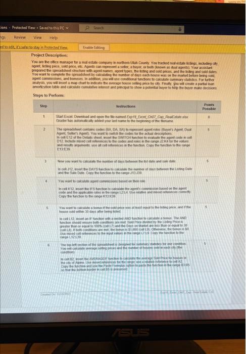
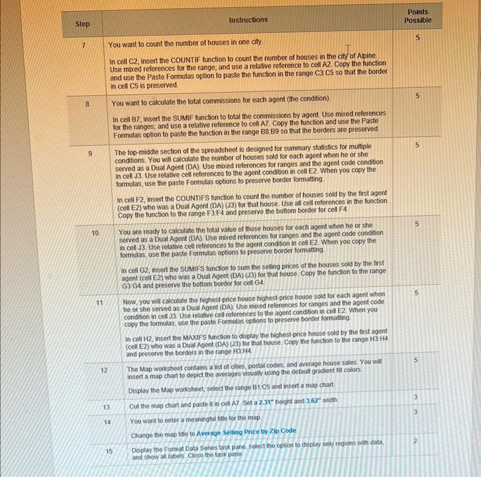
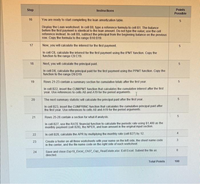
- Protected Virw - Stume to tha PC + (4.) Revew Vea Hip: Project Description: Steps to Perfors: 5 ilce mondeat 5 cendton Points Instructions Step Possible 7 You want to count the number of houses in one city. In cell C2, insert the COUNTIF function to count the number of houses in the city of Alpine. Use mbeed references for the range; and use a relative reference to cell A2. Copy the function and use the Paste Formulas option to paste the function in the range C3. C5 so that the border in cell C5 is preserved. 8 You want to calculate the fotal commissions for each agent (the condtion). 5 In cel B7, insert the SUMIF function to total the commissions by agent. Use mixed references for the ranges, and use a relative reference to cell A7. Copy the function and use the Paste Formulas option to paste the function in the range B8:B9 so that the borders are preserved. 9 The top-middle section of the spreadsheet is designed for summary statistics for muttiple condtions. You will calculate the number of houses sold for each agent when he or she served as a Dual Agent (DA). Use mixed references for ranges and the agent code condition in cell 3. Use relative cell references to the agent condition in cell E2. When you copy the formulas, use the paste Formulas options to preserve border formating. In cell F2, insert the COUNTIFS function to count the number of houses sold by the first agent (cell E2) who was a Dual Agent (DA) (J3) for that house. Use all cell references in the function. Copy the function to the range F3;F4 and preserve the bottom border for cell F4 10 You are ready to calculate the total value of those houses for each agent when he of she served as a Dual Agent (DA) Use mored references for ranges and the agent code condition in cel J. Use telative cell references to the agent condition in cell E2. When you copy the formulas, use the paste Formulas options to preserve border formatting. In cell G2, insert the SUMIFS function to sum the selling prices of the houses sold by the first agent (cell E2) who was a Dual Agent (DA) (J3) for that house Copy the function to the range G3 G4 and preserve the bottom border for cell G4 11 Now, you will calculate the highest-price house highest-price house sold for each agent when he or she served as a Dual Agent (DA). Use moced references for ranges and the agent code condition in cell J3. Use relative cell reterences to the agent condition in cell E2. When you copy the formulas, use the paste Formulas coptions to preserve border formatting. In cell H, insert the MAXIFS function to display the highest-price house sold by the first agent (cel E2) who was a Dual Agent (DA) (J3) for that house. Copy the function to the range H3.H4 and preserve the borders in the range H3H4. 12. The Map worksheet contains a list of cities, postal codes, and average house sales. You wil 5 insert a map chart to depict the averages visually using the defaul gradient fill colors. Display the Map worksheet, select the range B1,C5 and insert a map chart. 13. Cut the map chart and paste it in cell A7. Set a 2.31" height and 3.62width. 14 You want to enter a meaningtul titfe for the map. Change the map titie to Average Seiling Price by Zp Code. 2 15 Display the format Data Seties task pane, solect the optiont to display only regions with data. and show all labels. Close the task pane. Points Possible Display the Loan worksheet. In cell B8, type a reference formula to cell B1. The balance before the first payment is identical to the loan amount. Do not type the value; use the cell reference instead. In cell B9, subtract the principal from the beginning balance on the previous row. Copy the formula to the range B10.B19. 17 Now, you will calculate the interest for the first payment. In cell C8, calculate the interest for the first payment using the IPMT function. Copy the function to the range C9C19. 18 Next, you will calculate the principal paid. 5 In cell D8, caiculate the principal paid for the first payment using the PPMT function. Copy the function to the range D9:D19. 19 Rows 21-23 contain a summary section for cumulative totals after the first year. 5 In cell B22, insert the CUMIPMT function that calculates the cumulative interest after the first year. Use references to cells AB and A19 for the period arguments. 20 The next summary statistic will calculate the principal paid after the first year. 5 In cell B23, insert the CUMPRINC function that calculates the cumulative principal paid after the first year. Use references to cells A8 and A19 for the period arguments. 21 Rows 25-28 contain a section for what 4 analysis. 5 In cell B27, use the RATE financial function to calculate the periodic rate using $1,400 as the monthly payment (cell B26), the NPER, and loan amount in the original input section. 22 In cell B28, calculate the APR by muliplying the monthly rate (ces B27) by 12 . 23 Create a footer on all three worksheets with your name on the lett side, the sheet name code. in the center, and the fle name code on the right side of each worksheet 24 Save and cose Exp19_Excel_Cho7_Cap_Reaikstate xisx. Exot Excel. Submit the file as 0. directed Total Points 100