I need help understanding how to properly do thr calculations for the excel spreadsheet in the second photo. The first photo is a list of helpful hints. The last two photos are from the case study. please help fill in everything in the spreadsheet!

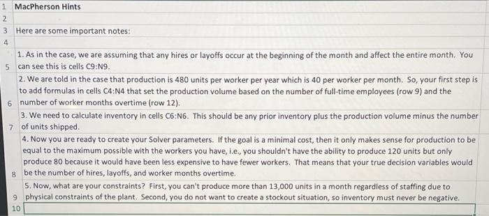
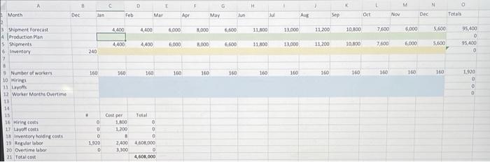
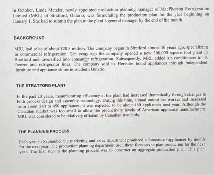
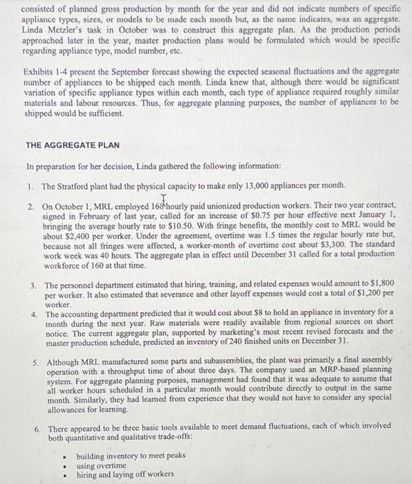
1 MacPherson Hints 2 3 Here are some important notes: 4 1. As in the case, we are assuming that any hires or layoffs occur at the beginning of the month and affect the entire month. You 5 can see this is cells C9:N9. 2. We are told in the case that production is 480 units per worker per year which is 40 per worker per month. So, your first step is to add formulas in cells C4:N4 that set the production volume based on the number of full-time employees (row 9) and the 6 number of worker months overtime (row 12). 3. We need to calculate inventory in cells C6:N6. This should be any prior inventory plus the production volume minus the number 7 of units shipped. 4. Now you are ready to create your Solver parameters. If the goal is a minimal cost, then it only makes sense for production to be equal to the maximum possible with the workers you have, i.e., you shouldn't have the ability to produce 120 units but only produce 80 because it would have been less expensive to have fewer workers. That means that your true decision variables would 8 be the number of hires, layoffs, and worker months overtime. 5. Now, what are your constraints? First, you can't produce more than 13,000 units in a month regardless of staffing due to 9 physical constraints of the plant. Second, you do not want to create a stockout situation, so inventory must never be negative. 10. A Month 3 Shipment Forecast 4 Production Plan 5 Shipments 6 Inventory 7 A 9 Number of workers 10 Hirings 11 Layoffs 12 Worker Months Overtime 13 14 15 16 Hiring costs 17 Layoff costs 18 Inventory holding costs 19 Regular labor 20 Overtime labor 21 Total cost Dec B Jan 240 160 W 1,920 C Feb D Mar 4,400 4,400 160 Cint per 1,800 1,200 B 0 2,400 4,608,000 3,300 4,608,000 4,400 4,400 160 Total 0 0 E Apr 6,000 6,000 160 F 8,000 8.000 160 May G 6,600 6,600 Jun 160 H 11,800 11800 160 Jul 1 13,000 13,000 160 Aug } 11,200 11,200 160 Sep K 10,800 10.800 160 Oct L 7,600 7,600 160 Nov M 6,000 6,000 160 Dec N 5,600 5,600 160 0 Total 95,400 D 95,400 0 1920 0 O 0 In October, Linda Metzler, newly appointed production planning manager of MacPherson Refrigeration Limited (MRL) of Stratford, Ontario, was formulating the production plan for the year beginning on January 1. She had to submit the plan to the plant's general manager by the end of the month. BACKGROUND MRL had sales of about $28.5 million. The company began in Stratford almost 30 years ago, specializing in commercial refrigeration. Ten years ago the company opened a new 300,000 square foot plant in Stratford and diversified into consumer refrigeration. Subsequently, MRL added air conditioners to its freezer and refrigerator lines. The company sold its Hercules brand appliances through independent furniture and appliance stores in southern Ontario. THE STRATFORD PLANT In the past 20 years, manufacturing efficiency at the plant had increased dramatically through changes in both process design and assembly technology. During this time, annual output per worker had increased from about 240 to 450 appliances; it was expected to be about 480 appliances next year. Although the Canadian market was too small to allow the productivity levels of American appliance manufacturers, MRL was considered to be relatively efficient by Canadian standards. THE PLANNING PROCESS Each year in September the marketing and sales department produced a forecast of appliances by month for the next year. The production planning department used these forecasts to plan production for the next year. The first step in the planning process was to construct an aggregate production plan. This plan consisted of planned gross production by month for the year and did not indicate numbers of specific appliance types, sizes, or models to be made each month but, as the name indicates, was an aggregate. Linda Metzler's task in October was to construct this aggregate plan. As the production periods approached later in the year, master production plans would be formulated which would be specific regarding appliance type, model number, etc. Exhibits 1-4 present the September forecast showing the expected seasonal fluctuations and the aggregate number of appliances to be shipped each month. Linda knew that, although there would be significant variation of specific appliance types within each month, each type of appliance required roughly similar materials and labour resources. Thus, for aggregate planning purposes, the number of appliances to be shipped would be sufficient. THE AGGREGATE PLAN In preparation for her decision, Linda gathered the following information: 1. The Stratford plant had the physical capacity to make only 13,000 appliances per month. 2. On October 1, MRL employed 16 hourly paid unionized production workers. Their two year contract, signed in February of last year, called for an increase of $0.75 per hour effective next January 1, bringing the average hourly rate to $10.50. With fringe benefits, the monthly cost to MRL would be about $2,400 per worker. Under the agreement, overtime was 1.5 times the regular hourly rate but, because not all fringes were affected, a worker-month of overtime cost about $3,300. The standard work week was 40 hours. The aggregate plan in effect until December 31 called for a total production workforce of 160 at that time. 3. The personnel department estimated that hiring, training, and related expenses would amount to $1,800 per worker. It also estimated that severance and other layoff expenses would cost a total of $1,200 per worker. 4. The accounting department predicted that it would cost about $8 to hold an appliance in inventory for a month during the next year. Raw materials were readily available from regional sources on short notice. The current aggregate plan, supported by marketing's most recent revised forecasts and the master production schedule, predicted an inventory of 240 finished units on December 31. 5. Although MRL manufactured some parts and subassemblies, the plant was primarily a final assembly operation with a throughput time of about three days. The company used an MRP-based planning system. For aggregate planning purposes, management had found that it was adequate to assume that all worker hours scheduled in a particular month would contribute directly to output in the same month. Similarly, they had learned from experience that they would not have to consider any special allowances for learning. 6. There appeared to be three basic tools available to meet demand fluctuations, each of which involved both quantitative and qualitative trade-offs: building inventory to meet peaks using overtime hiring and laying off workers