I need help with understanding and how to do the data analysis on excel. The data is from SHINY

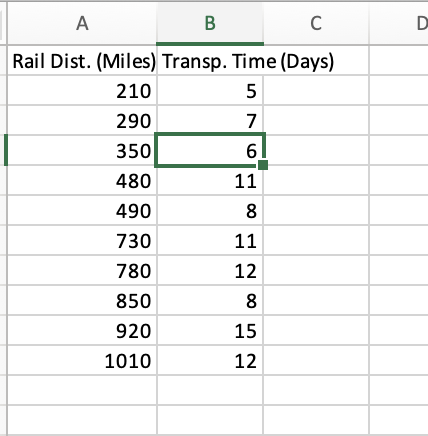
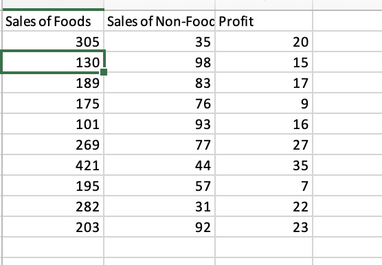
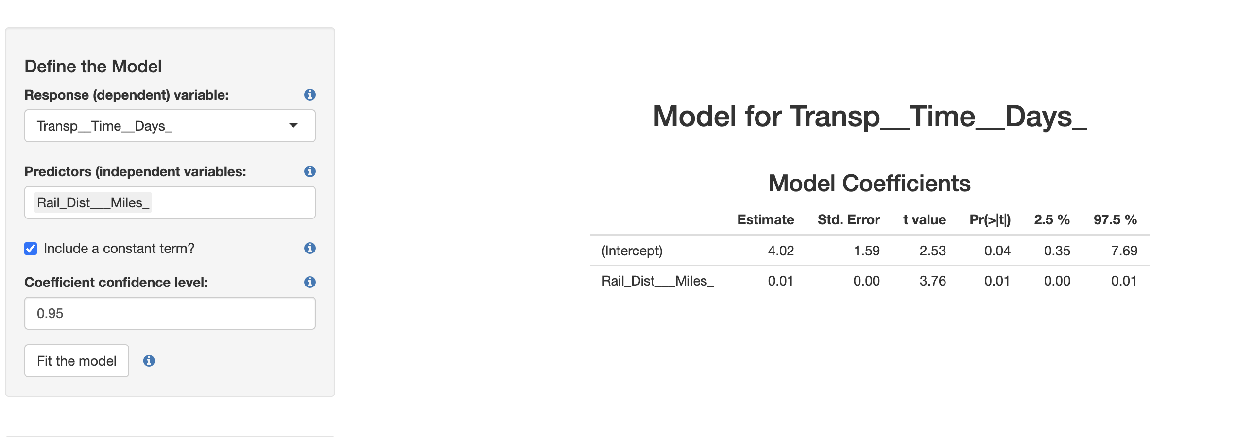
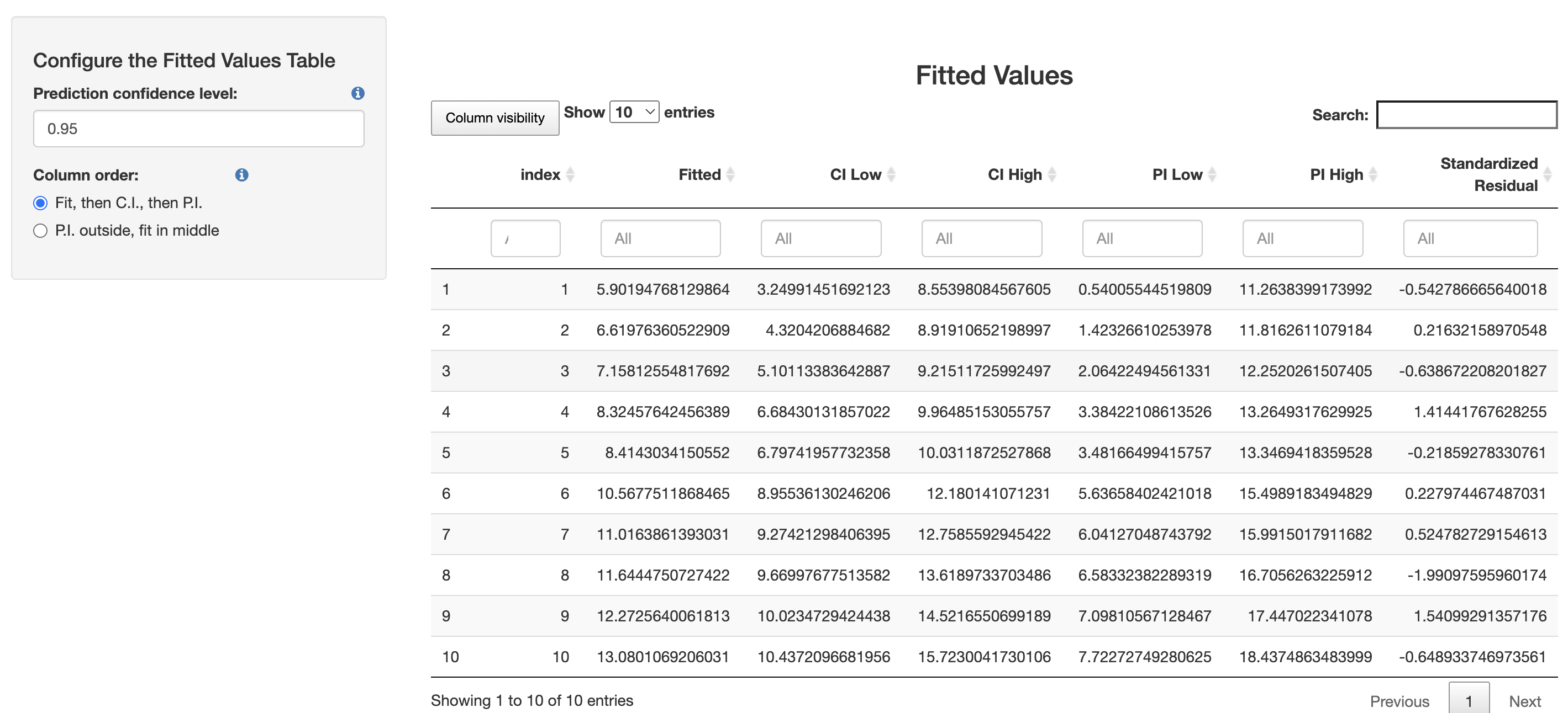
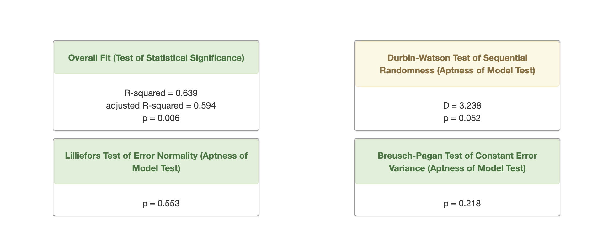
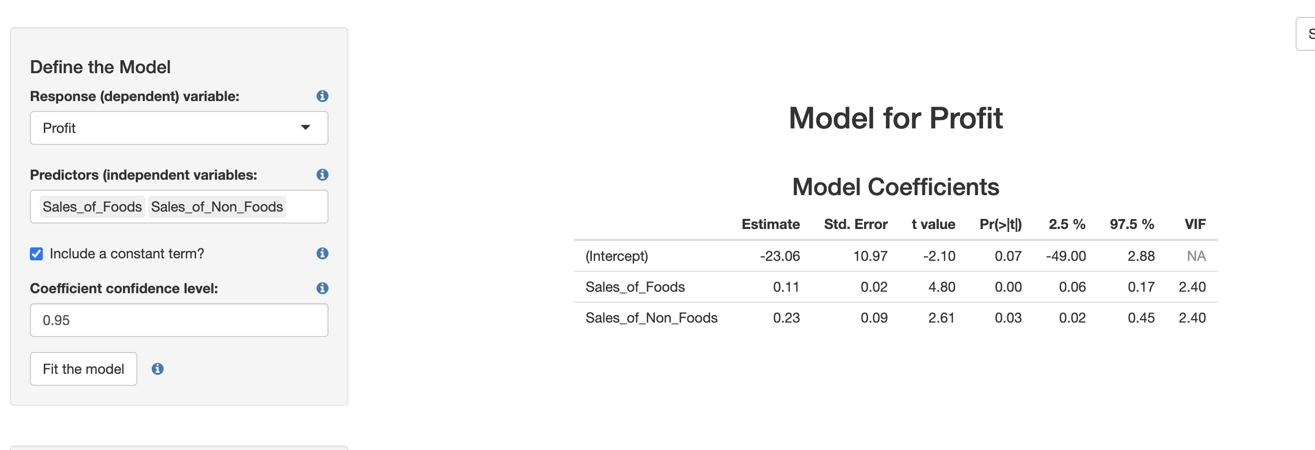
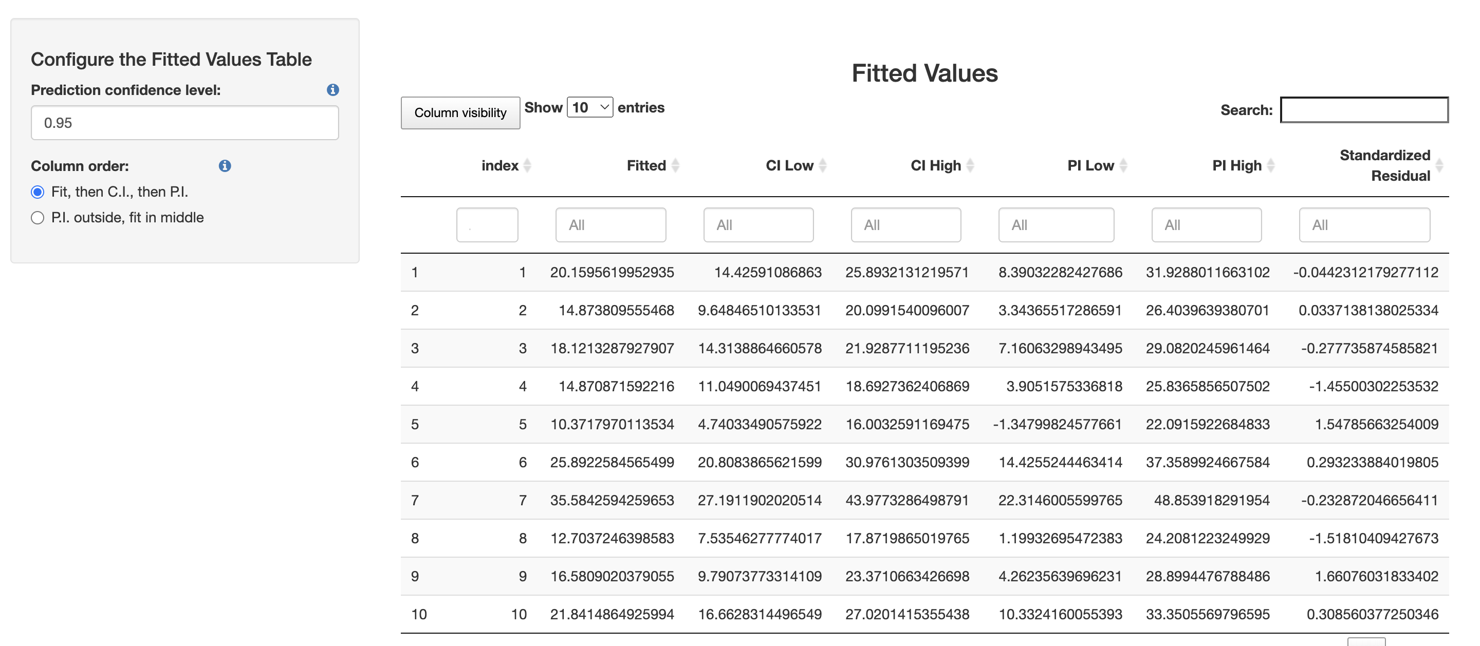
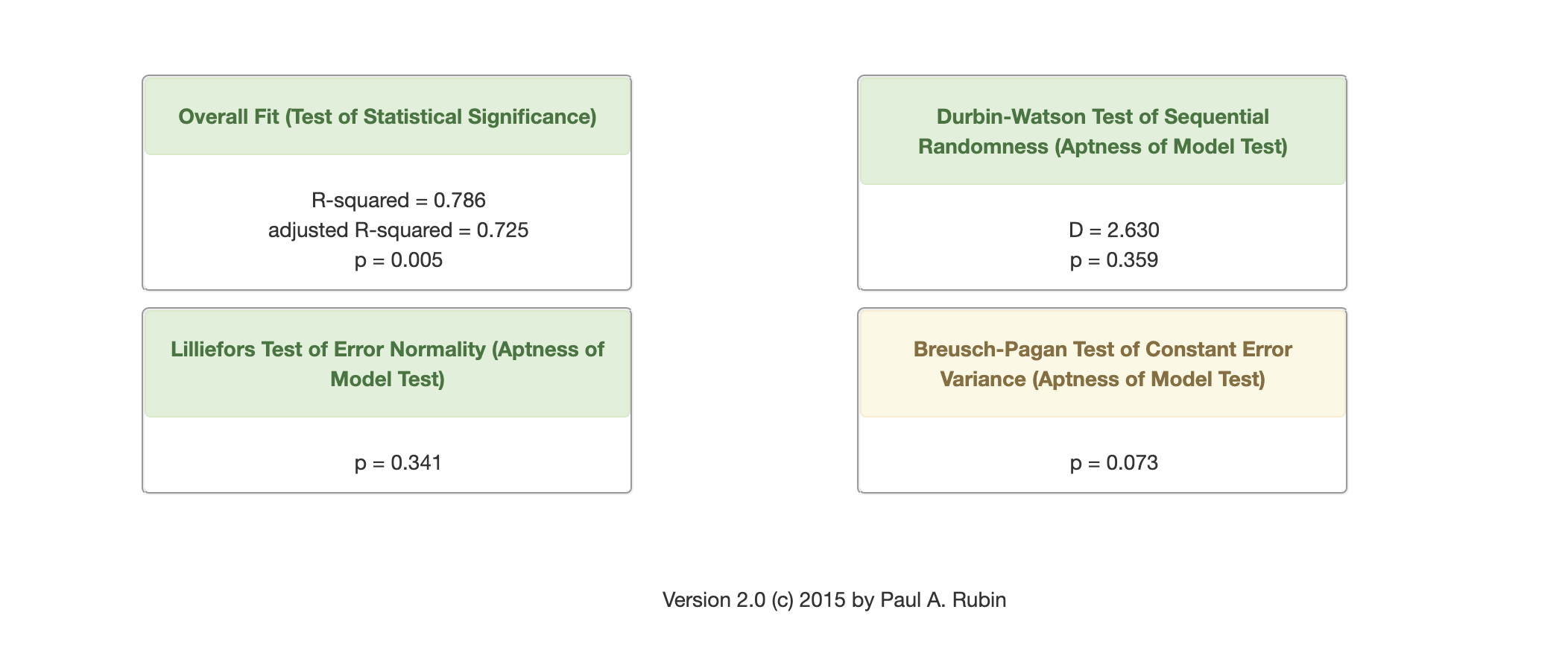
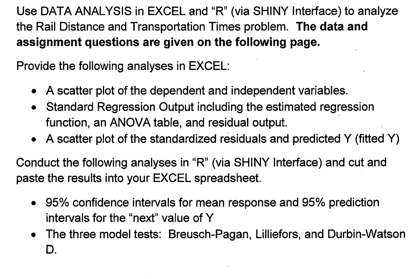
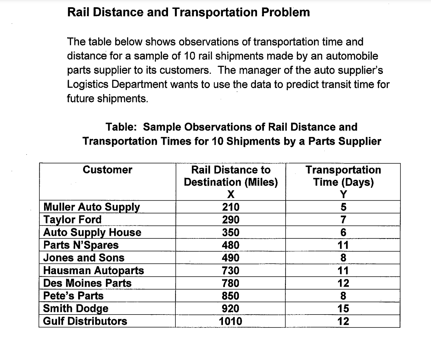
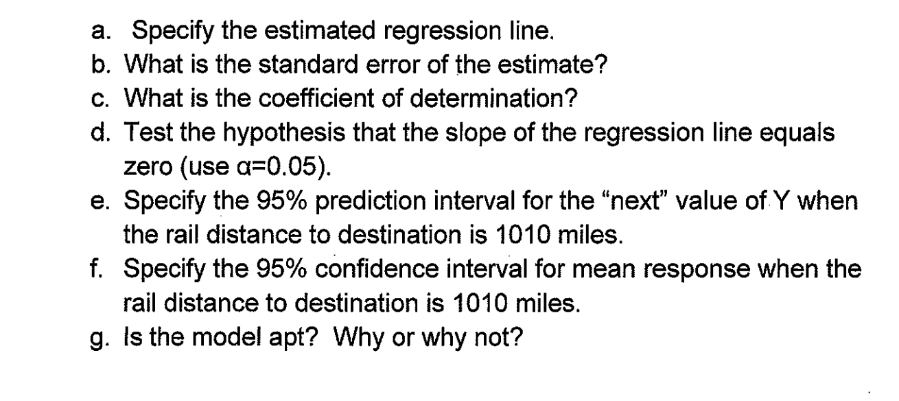
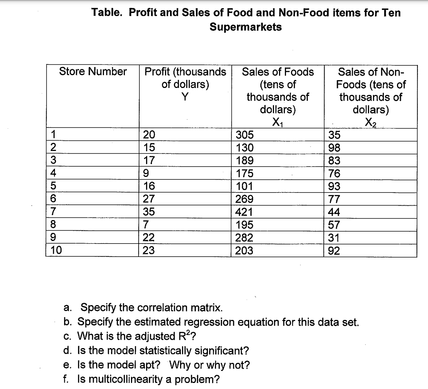
\f\fDefine the Model Response (dependent) variable: Transp_Time_Days_ Model for Transp_Time_Days_ Predictors (independent variables: i Model Coefficients Rail_Dist_Miles_ Estimate Std. Error t value Pr(>|t)) 2.5 % 97.5 % Include a constant term? i (Intercept) 4.02 1.59 2.53 0.04 0.35 7.69 Coefficient confidence level: Rail_Dist Miles_ 0.01 0.00 3.76 0.01 0.00 0.01 0.95 Fit the modelConfigure the Fitted Values Table Fitted Values Prediction confidence level: i Column visibility Show 10 entries Search: 0.95 Column order: index Fitted CI Low CI High PI Low PI High Standardized Residual O Fit, then C.I., then P.I. O P.I. outside, fit in middle All All All All All All 1 1 5.90194768129864 3.24991451692123 8.55398084567605 0.54005544519809 11.2638399173992 -0.542786665640018 2 2 6.61976360522909 4.3204206884682 8.91910652198997 1.42326610253978 11.8162611079184 0.21632158970548 3 3 7.15812554817692 5.10113383642887 9.21511725992497 2.06422494561331 12.2520261507405 -0.638672208201827 4 4 8.32457642456389 6.68430131857022 9.96485153055757 3.38422108613526 13.2649317629925 1.41441767628255 5 5 8.4143034150552 6.79741957732358 10.0311872527868 3.48166499415757 13.3469418359528 -0.21859278330761 6 6 10.5677511868465 8.95536130246206 12.180141071231 5.63658402421018 15.4989183494829 0.227974467487031 7 7 11.0163861393031 9.27421298406395 12.7585592945422 6.04127048743792 15.9915017911682 0.524782729154613 8 8 11.6444750727422 9.66997677513582 13.6189733703486 6.58332382289319 16.7056263225912 -1.99097595960174 9 9 12.2725640061813 10.0234729424438 14.5216550699189 7.09810567128467 17.447022341078 1.54099291357176 10 10 13.0801069206031 10.4372096681956 15.7230041730106 7.72272749280625 18.4374863483999 -0.648933746973561 Showing 1 to 10 of 10 entries Previous NextOverall Fit (Test of Statistical Significance) Durbin-Watson Test of Sequential Randomness (Aptness of Model Test) Rsquared = 0.639 adjusted Rsquared = 0.594 D = 3.238 p = 0.006 p = 0.052 Lilliefors Test of Error Normality (Aptness of Breusch-Pagan Test of Constant Error Model Test) Variance (Aptness of Model Test) p = 0.553 p = 0.218 Define the Model Response (dependent) variable: i Profit Model for Profit Predictors (independent variables: Model Coefficients Sales_of_Foods Sales_of_Non_Foods Estimate Std. Error t value Pr(>|t) 2.5 % 97.5 % VIF Include a constant term? (Intercept) -23.06 10.97 -2.10 0.07 -49.00 2.88 NA Coefficient confidence level: Sales_of_Foods 0.11 0.02 4.80 0.00 0.06 0.17 2.40 0.95 Sales_of_Non_Foods 0.23 0.09 2.61 0.03 0.02 0.45 2.40 Fit the model iConfigure the Fitted Values Table Fitted Values Prediction confidence level: i Column visibility Show 10 entries Search: 0.95 Standardized Column order: index Fitted CI Low CI High PI Low PI High Residual O Fit, then C.I., then P.I. O P.I. outside, fit in middle All All All All All All 1 1 20.1595619952935 14.42591086863 25.8932131219571 8.39032282427686 31.9288011663102 -0.0442312179277112 2 2 14.873809555468 9.64846510133531 20.0991540096007 3.34365517286591 26.4039639380701 0.0337138138025334 3 3 18.1213287927907 14.3138864660578 21.9287711195236 7.16063298943495 29.0820245961464 -0.277735874585821 4 4 14.870871592216 11.0490069437451 18.6927362406869 3.9051575336818 25.8365856507502 -1.45500302253532 5 10.3717970113534 4.74033490575922 16.0032591169475 -1.34799824577661 22.0915922684833 1.54785663254009 6 6 25.8922584565499 20.8083865621599 30.9761303509399 14.4255244463414 37.3589924667584 0.293233884019805 7 7 35.5842594259653 27.1911902020514 43.9773286498791 22.3146005599765 48.853918291954 -0.232872046656411 8 8 12.7037246398583 7.53546277774017 17.8719865019765 1.19932695472383 24.2081223249929 -1.51810409427673 9 9 16.5809020379055 9.79073773314109 23.3710663426698 4.26235639696231 28.8994476788486 1.66076031833402 10 10 21.8414864925994 16.6628314496549 27.0201415355438 10.3324160055393 33.3505569796595 0.308560377250346Overall Fit (Test of Statistical Significance) Durbin-Watson Test of Sequential Randomness (Aptness of Model Test) R-squared = 0.786 adjusted R-squared = 0.725 D = 2.630 p = 0.005 p = 0.359 Lilliefors Test of Error Normality (Aptness of Breusch-Pagan Test of Constant Error Model Test) Variance (Aptness of Model Test) P = 0.341 p = 0.073 Version 2.0 (c) 2015 by Paul A. RubinUse DATA ANALYSIS in EXCEL and \"R\" (via SHINY Interface) to analyze the Rail Distance and Transportation Times problem. The data and assignment questions are given on the following page. Provide the following analyses in EXCEL: o A scatter plot of the dependent and independent variables. 0 Standard Regression Output including the estimated regression function, an ANOVA table and residual output. 0 A scatter plot of the standardized residuals and predicted Y (fitted Y) Conduct the following analyses in "R\" (via SHINY Interface) and cut and paste the results into your EXCEL spreadsheet. - 95% confidence intervals for mean response and 95% prediction intervals for the \"next\" value of Y o The three model tests: Breusch-Pagan, Lilliefors, and Durbin-Watson D. Rail Distance and Transportation Problem The table below shows observations of transportation time and distance for a sample of to rail shipments made by an automobile parts supplier to its customers. The manager of the auto supplier's Logistics Department Wants to use the data to predict transit time for future shipments. Table: Sample Observations of Rail Distance and Transportation Times for 10 Shipments by a Parts Supplier Customer Rail Distance to Transportation Destination (Miles) Time (Days) m -E_ . Muller Auto Su . ni Auto Su- I House \"- ___I_ -EI-- -_E_ __ _- __ -_ Des Moines Parts Pete's Parts .5- Smith Dod-e .255- -E_ Gulf Distributors a. Specify the estimated regression line. b. What is the standard error of the estimate? c. What is the coefficient of determination? d. Test the hypothesis that the slope of the regression line equals zero (use (1:005). e. Specify the 95% prediction interval for the \"next\" value of-Y when the rail distance to destination is 1010 miles. f. Specify the 95% confidence interval for mean response when the rail distance to destination is 1010 miles. g. is the model apt? Why or why not? Table. Profit and Sales of Food and Non-Food items for Ten Supermarkets Sales of Non- Foods (tens of thousands of dollars) Sales of Foods (tens of thousands of dollars) Store Number Profit (thousands of dollars) a. Specify the correlation matrix. - b. Specify the estimated regression equation for this data set. c. What is the adjusted R2? d. is the model statistically significant? e. Is the model apt? "Why or why not? f. Is multicollinearity a problem? Use DATA ANALYSIS in EXCEL and "R\" (via SHINY Interface) to analyze the Profit and Sales of Food and Nonfood problem. The data and assignment questions are given on the following page. Provide the following analyses in EXCEL: o A correlation matrix for all variables. 0 Scatter plots of the dependent variable and each independent variable. 0 Standard Regression Output including the estimated regression function, an ANOVA table, and residual output. 0 A scatter plot of the standardized residuals and predicted Y (fitted Y) . The VIP for each independent variable. Conduct the following analyses in \"R\" (via SHlNY interface) and cut and paste the results into your EXCEL spreadsheet. o The three model tests: Breusch-Pagan, Lilliefors,'and Durbin-Watson D