I NEED it completed in CELL REFERENCE FORMAT.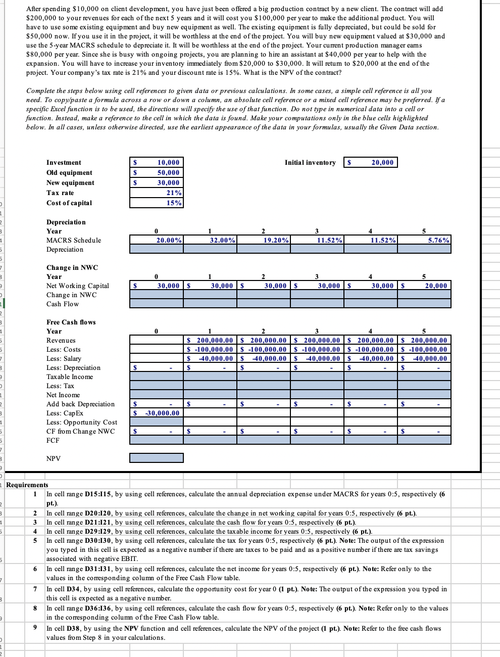

After spending $10,000 on client development, you have just been offered a big production contract by a new client. The contract will add $200,000 to your revenues for each of the next 5 years and it will cost you $ 100,000 per year to make the additional product. You will have to use some existing equipment and buy new equipment as well. The existing equipment is fully depreciated, but could be sold for $50,000 now. If you use it in the project, it will be worthless at the end of the project. You will buy new equipment valued at $30,000 and use the 5-year MACRS schedule to depreciate it. It will be worthless at the end of the project. Your current production manager earns $80,000 per year. Since she is busy with ongoing projects, you are planning to hire an assistant at $40,000 per year to help with the expansion. You will have to increase your inventory immediately from $20,000 to $30,000. It will retum to $20,000 at the end of the project. Your company's tax rate is 21% and your discount rate is 15%. What is the NPV of the contract? Complete the steps below using cell references to given data or previous calculations. In some cases, a simple cell reference is all you need. To copy/paste a formula across row or down a column, an absolute cell reference or a mixed cell reference may be preferred. If a specific Excel function is to be used, the directions will specify the use of that function. Do not type in numerical data into a cell or function. Instead, make a reference to the cell in which the data is found. Make your computations only in the blue cells highlighted below. In all cases, unless otherwise directed, use the earliest appearance of the data in your formulas, usually the Given Data section. $ 10,000 Initial inventory $ 20,000 $ Investment Old equipment New equipment Tax rate Cost of capital $ 50,000 30,000 21% 15% Depreciation Year MACRS Schedule Depreciation 1 32.00% 2 19.20% 3 11.52% 20.00% 11.52% 5 5.76% Change in NWC Year Net Working Capital Change in NWC Cash Flow 0 30,000$ 1 30,000 $ 2 30,000 $ 3 30,000 $ 4 30,000 $ 5 20,000 $ 0 2 3 4 5 $ 200,000.00 $ 200,000.00 $ 200,000.00 $ 200,000.00 $ 200,000.00 $ -100,000.00 $ -100,000.00 $ -100,000.00 $ -100,000.00 $ -100,000.00 $ -40,000.00 $ 40,000.00 $ -40,000.00 $ 40,000.00 $ -40,000.00 $ $ S $ $ $ Free Cash flows Year Revenues Less: Costs Less: Salary Less: Depreciation Taxable income Less: Tax Net Income Add back Depreciation Less: Cap Ex Less: Opportunity Cost CF from Change NWC FCF $ $ $ -30,000.00 $ $ $ $ $ NPV 2 3 2 5 4 Requirements 1 In cell range D15:115, by using cell references, calculate the annual depreciation expense under MACRS for years 0:5, respectively (6 pt.) In cell range D20:120, by using cell references, calculate the change in net working capital for years 0:5, respectively (6 pt.). 3 In cell range D21:121, by using cell references, calculate the cash flow for years 0:5, respectively (6 pt.). In cell range D29:129, by using cell references, calculate the taxable income for years 0:5, respectively (6 pt.). 5 In cell range D30:130, by using cell references, calculate the tax for years 0:5, respectively (6 pt.). Note: The output of the expression you typed in this cell is expected as a negative number if there are taxes to be paid and as a positive number if there are tax savings associated with negative EBIT. In cell range D31:131, by using cell references, calculate the net income for years 0:5, respectively 6 pt.). Note: Refer only to the values in the corresponding column of the Free Cash Flow table. In cell D34, by using cell references, calculate the opportunity cost for year 0 (1 pt.). Note: The output of the expression you typed in this cell is expected as a negative number. In cell range D36:136, by using cell references, calculate the cash flow for years 0:5, respectively (6 pt.). Note: Refer only to the values in the corresponding column of the Free Cash Flow table. In cell D38, by using the NPV function and cell references, calculate the NPV of the project (1 pt.). Note: Refer to the free cash flows values from Step 8 in your calculations. 6 7 7 3 8 9 After spending $10,000 on client development, you have just been offered a big production contract by a new client. The contract will add $200,000 to your revenues for each of the next 5 years and it will cost you $ 100,000 per year to make the additional product. You will have to use some existing equipment and buy new equipment as well. The existing equipment is fully depreciated, but could be sold for $50,000 now. If you use it in the project, it will be worthless at the end of the project. You will buy new equipment valued at $30,000 and use the 5-year MACRS schedule to depreciate it. It will be worthless at the end of the project. Your current production manager earns $80,000 per year. Since she is busy with ongoing projects, you are planning to hire an assistant at $40,000 per year to help with the expansion. You will have to increase your inventory immediately from $20,000 to $30,000. It will retum to $20,000 at the end of the project. Your company's tax rate is 21% and your discount rate is 15%. What is the NPV of the contract? Complete the steps below using cell references to given data or previous calculations. In some cases, a simple cell reference is all you need. To copy/paste a formula across row or down a column, an absolute cell reference or a mixed cell reference may be preferred. If a specific Excel function is to be used, the directions will specify the use of that function. Do not type in numerical data into a cell or function. Instead, make a reference to the cell in which the data is found. Make your computations only in the blue cells highlighted below. In all cases, unless otherwise directed, use the earliest appearance of the data in your formulas, usually the Given Data section. $ 10,000 Initial inventory $ 20,000 $ Investment Old equipment New equipment Tax rate Cost of capital $ 50,000 30,000 21% 15% Depreciation Year MACRS Schedule Depreciation 1 32.00% 2 19.20% 3 11.52% 20.00% 11.52% 5 5.76% Change in NWC Year Net Working Capital Change in NWC Cash Flow 0 30,000$ 1 30,000 $ 2 30,000 $ 3 30,000 $ 4 30,000 $ 5 20,000 $ 0 2 3 4 5 $ 200,000.00 $ 200,000.00 $ 200,000.00 $ 200,000.00 $ 200,000.00 $ -100,000.00 $ -100,000.00 $ -100,000.00 $ -100,000.00 $ -100,000.00 $ -40,000.00 $ 40,000.00 $ -40,000.00 $ 40,000.00 $ -40,000.00 $ $ S $ $ $ Free Cash flows Year Revenues Less: Costs Less: Salary Less: Depreciation Taxable income Less: Tax Net Income Add back Depreciation Less: Cap Ex Less: Opportunity Cost CF from Change NWC FCF $ $ $ -30,000.00 $ $ $ $ $ NPV 2 3 2 5 4 Requirements 1 In cell range D15:115, by using cell references, calculate the annual depreciation expense under MACRS for years 0:5, respectively (6 pt.) In cell range D20:120, by using cell references, calculate the change in net working capital for years 0:5, respectively (6 pt.). 3 In cell range D21:121, by using cell references, calculate the cash flow for years 0:5, respectively (6 pt.). In cell range D29:129, by using cell references, calculate the taxable income for years 0:5, respectively (6 pt.). 5 In cell range D30:130, by using cell references, calculate the tax for years 0:5, respectively (6 pt.). Note: The output of the expression you typed in this cell is expected as a negative number if there are taxes to be paid and as a positive number if there are tax savings associated with negative EBIT. In cell range D31:131, by using cell references, calculate the net income for years 0:5, respectively 6 pt.). Note: Refer only to the values in the corresponding column of the Free Cash Flow table. In cell D34, by using cell references, calculate the opportunity cost for year 0 (1 pt.). Note: The output of the expression you typed in this cell is expected as a negative number. In cell range D36:136, by using cell references, calculate the cash flow for years 0:5, respectively (6 pt.). Note: Refer only to the values in the corresponding column of the Free Cash Flow table. In cell D38, by using the NPV function and cell references, calculate the NPV of the project (1 pt.). Note: Refer to the free cash flows values from Step 8 in your calculations. 6 7 7 3 8 9