I would like to summarize this section, with an example for clarification, please

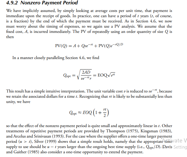
4.9.2 Nonzero Payment Period We have implicitly assumed, by simply looking at average costs per unit time, that payment is immediate upon the receipt of goods. In practice, one can have a period of t years ( t, of course, is a fraction) by the end of which the payment must be received. As in Section 4.6, we now must worry about the timing of expenses, so we again use a PV analysis. We assume that the fixed cost, A, is incurred immediately. The PV of repeatedly using an order quantity of size Q is then PV(Q)=A+Qvert+PV(Q)erQ/D In a manner closely paralleling Section 4.6, we find Qopt=ver2AD=EOQent This result has a simple intuitive interpretation. The unit variable cost v is reduced to vert, because we retain the associated dollars for a time t. Recognizing that rt is likely to be substantially less than unity, we have QoptEOQ(1+2rt) so that the effect of the nonzero payment period is quite small and approximately linear in t. Other treatments of repetitive payment periods are provided by Thompson (1975), Kingsman (1983), and Arcelus and Srinivasan (1993). For the case where the supplier offers a one-time larger payment period (u>t), Silver (1999) shows that a simple result holds, namely that the appropriate time/ate supply to use should be ut years larger than the ongoing best time supply (i.e., Qopt/D ). Davis Settir and Gaither (1985) also consider a one-time opportunity to extend the payment. 4.9.2 Nonzero Payment Period We have implicitly assumed, by simply looking at average costs per unit time, that payment is immediate upon the receipt of goods. In practice, one can have a period of t years ( t, of course, is a fraction) by the end of which the payment must be received. As in Section 4.6, we now must worry about the timing of expenses, so we again use a PV analysis. We assume that the fixed cost, A, is incurred immediately. The PV of repeatedly using an order quantity of size Q is then PV(Q)=A+Qvert+PV(Q)erQ/D In a manner closely paralleling Section 4.6, we find Qopt=ver2AD=EOQent This result has a simple intuitive interpretation. The unit variable cost v is reduced to vert, because we retain the associated dollars for a time t. Recognizing that rt is likely to be substantially less than unity, we have QoptEOQ(1+2rt) so that the effect of the nonzero payment period is quite small and approximately linear in t. Other treatments of repetitive payment periods are provided by Thompson (1975), Kingsman (1983), and Arcelus and Srinivasan (1993). For the case where the supplier offers a one-time larger payment period (u>t), Silver (1999) shows that a simple result holds, namely that the appropriate time/ate supply to use should be ut years larger than the ongoing best time supply (i.e., Qopt/D ). Davis Settir and Gaither (1985) also consider a one-time opportunity to extend the payment