Identify two different approaches to dealing with missing values.

In the space provided, identify and briefly describe the two approaches.

• A1. First Approach
• A2. Second Approach

Identify a significant similarity and a significant difference between A1 and A2:

• A. Similarity
• B. Difference
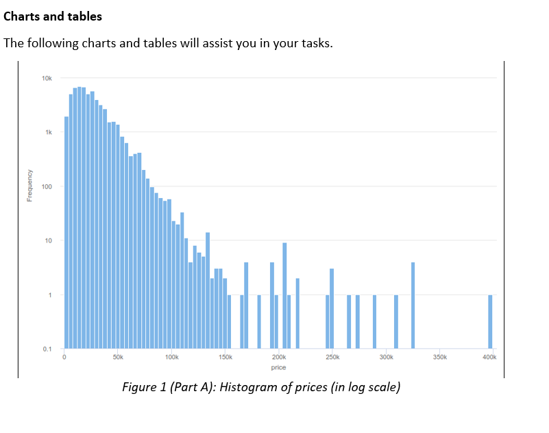
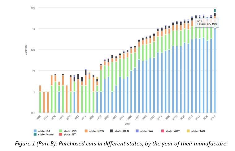
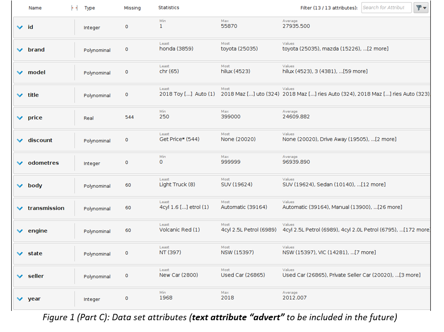
• Business Scenario: Second Hand Car Sales A large Australian second hand car dealer Pre-Loved Cars (P-LC), with dealerships across all Australian states, asked you to develop a method of estimating a purchase price of any new car brought into their dealerships. At the moment, each car is described using structured data only, which is based on the car detailed evaluation in one of their workshops. However, in the future P-LC would like to pro-actively seek business opportunities by identifying prospective clients personal advertising placed on social media. P-LC provided you with data of past car evaluations and would like you to clean-up and explore car data, develop and evaluate a model predicting their prices (label), and minimize the classification or estimation error in the process. They have already undertaken some model development and attached the preliminary results for your comment. In several cases, the original numeric label was discretised. Data P-LC provided you with a sample of 55,870 car evaluations, which include 13 attributes: car ID, brand, model and their popular name (title), type of discount given, odometer/mileage reading (kilometres), body type, transmission, engine, state where the acquisition was made (e.g. Victoria), seller type (e.g. Private Seller), year of car manufacturing and price (label). P-LC are also planning to include a new attribute advert to include text sourced from social media. Some attributes have missing values or outliers. Charts and tables The following charts and tables will assist you in your tasks.

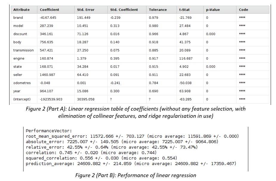
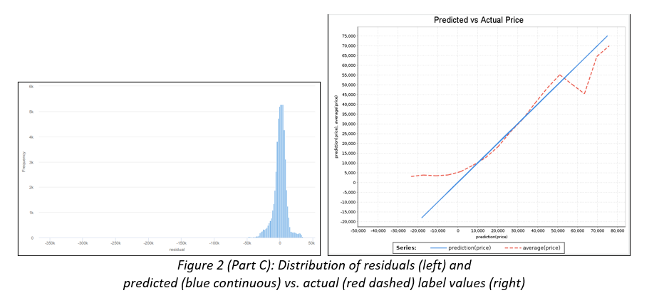
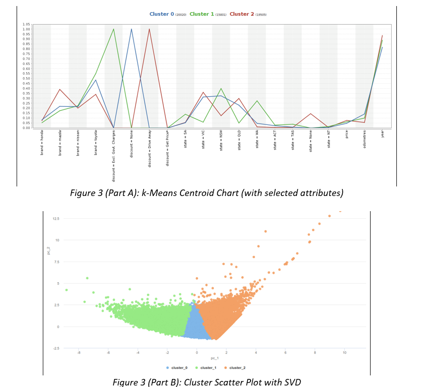
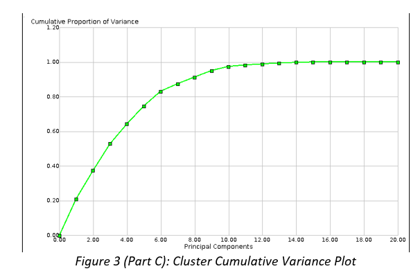
elimination of collinear features, and ridge regularisation in use) \begin{tabular}{|l} Performancevector: \\ root_mean_squared_error: 11572.666+/703.127 (micro average: 11591.869+/0.000 ) \\ absolute_error: 7225.007+/149.505 (micro average: 7225.007+/9064.806 ) \\ relative_error: 42.55%+/0.64% (micro average: 42.55%+/73.47% ) \\ correlation: 0.745+/0.020 (micro average: 0.744 ) \\ squared_correlation: 0.556+/0.030 (micro average: 0.554 ) \\ prediction_average: 24609.882+/214.859 (micro average: 24609.882+/17359.467 ) \end{tabular} Figure 2 (Part B): Performance of linear regression Figure 2 (Part C): Distribution of resduals (left) and predicted (blue continuous) vs. actual (red dashed) label values (right) Figure 1 (Part B): Purchased cars in different states, by the year of their manufacture Figure 1 (Part C): Data set attributes (text attribute "advert" to be included in the future) Figure 3 (Part C): Cluster Cumulative Variance Plot Figure 3 (Part A): k-Means Centroid Chart (with selected attributes) Figure 3 (Part B): Cluster Scatter Plot with SVD Charts and tables The following charts and tables will assist you in your tasks. elimination of collinear features, and ridge regularisation in use) \begin{tabular}{|l} Performancevector: \\ root_mean_squared_error: 11572.666+/703.127 (micro average: 11591.869+/0.000 ) \\ absolute_error: 7225.007+/149.505 (micro average: 7225.007+/9064.806 ) \\ relative_error: 42.55%+/0.64% (micro average: 42.55%+/73.47% ) \\ correlation: 0.745+/0.020 (micro average: 0.744 ) \\ squared_correlation: 0.556+/0.030 (micro average: 0.554 ) \\ prediction_average: 24609.882+/214.859 (micro average: 24609.882+/17359.467 ) \end{tabular} Figure 2 (Part B): Performance of linear regression Figure 2 (Part C): Distribution of resduals (left) and predicted (blue continuous) vs. actual (red dashed) label values (right) Figure 1 (Part B): Purchased cars in different states, by the year of their manufacture Figure 1 (Part C): Data set attributes (text attribute "advert" to be included in the future) Figure 3 (Part C): Cluster Cumulative Variance Plot Figure 3 (Part A): k-Means Centroid Chart (with selected attributes) Figure 3 (Part B): Cluster Scatter Plot with SVD Charts and tables The following charts and tables will assist you in your tasks