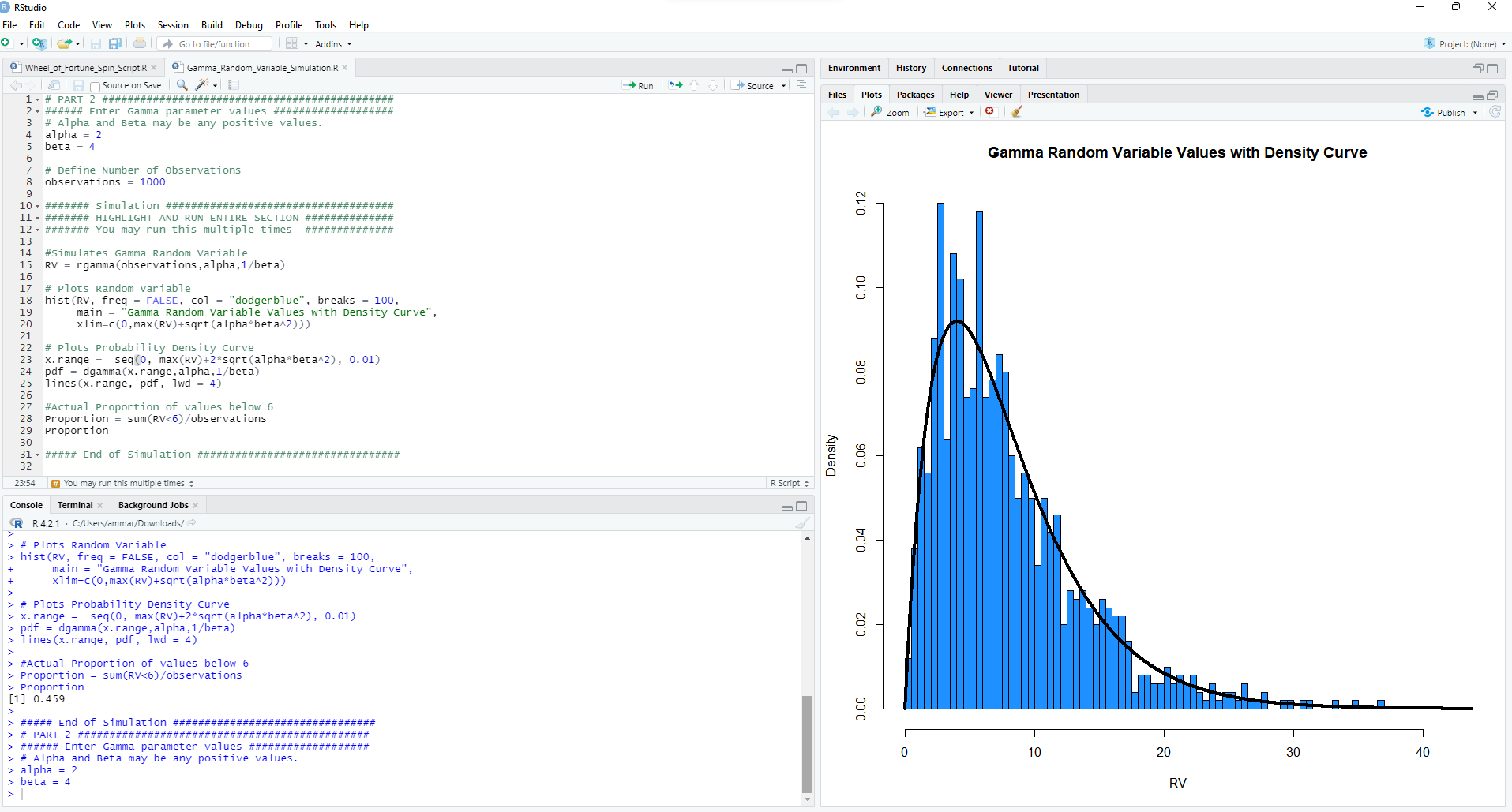
imulation of Gamma Random Variables Background: When we use the probability density function to find probabilities for a random variable, we are using the density function as a model. This is a smooth curve, based on the shape of observed outcomes for the random variable. The observed distribution will be rough and may not follow the model exactly. The probability density curve, or function, is still just a model for what is actually happening with the random variable. In other words, there can be some discrepancies between the actual proportion of values above x and the proportion of area under the curve above the same value x. Our expectation is as the number of observations increase, literally or theoretically, the observed distribution will align more with the density curve. Over the long run, the differences are negligible, the model is sufficient and more convenient to find desired information. Simulation: Use R to simulate 1000 observations from a gamma distribution. To begin, set alpha = 2 and beta = 4. Highlight and run the parameters and observation values. Run the simulation code to plot the observations and fit the probability density function over the observations. You don't need to change anything. You may run the section all at once by highlighting all of the section and running it by clicking the run button at the top of the script window. a. Given the values are from a gamma distribution with alpha= 2 and beta = 4, i. (1 points) What is the expression for the probability density function? ii. (1 point) What is the average and standard deviation of the random variable? Show work in regards to how you derived these quantities. iii. (1 point) What is the probability x is less than 6? Show work. b. (2 point) Run the simulation and paste your plot. Comment on the general shape of the distribution. How well does the density curve fit the observations? c. (2 point) What is the exact proportion of values below 6? How does the actual proportion compare to the probability from the density curve in part 2-a-ili?R RStudio X File Edit Code View Plots Session Build Debug Profile Tools Help . 0 3 .Ha| |Go to file/function 18: . Addins . R Project: (None) - 97 Wheel_of Fortune_Spin_Script.R x @ Gamma_Random_Variable_Simulation.R> Environment History Connections Tutorial Source on Save . Run # 1 3 Source . = 1. # PART 2 # ########### # # ## # # # # # # # # # # # # # # # # # # # # ## # # # # ### # Files Plots Packages Help Viewer Presentation 2 . ###### Enter Gamma parameter values ################ ### Zoom Export - Publish . C # Alpha and Beta may be any positive values. alpha = 2 beta = 6 Gamma Random Variable Values with Density Curve 7 # Define Number of observations 8 observations = 1000 9 10- ####### Simulation #################0################## 0.12 11 . ####### HIGHLIGHT AND RUN ENTIRE SECTION ############## 12 - ####### You may run this multiple times ############## 13 14 #Simulates Gamma Random Variable 15 RV = rgamma (observations , alpha, 1/beta) 16 17 # Plots Random Variable 0.10 18 hist (RV, freq = FALSE, col = "dodgerblue", breaks = 100, 19 main = "Gamma Random variable values with Density curve", 20 klim=c(0, max (RV)+sqrt (alpha*beta^2) )) 21 22 # Plots Probability Density Curve 23 x. range = seq(0, max(RV)+2*sqrt (alpha*beta^2) , 0. 01) 24 pdf = dgamma (x. range, alpha, 1/beta) 0.08 25 lines (x. range, pdf , 1wd = 4) 26 27 #Actual Proportion of values below 6 28 Proportion = sum(RV hist (RV, freq = FALSE, col = "dodgerblue", breaks = 100, main = "Gamma Random Variable values with Density curve", xlim=c(0, max (RV)+sqrt(alpha*beta^2))) # Plots Probability Density curve x. range = seq(0, max (RV)+2*sqrt (alpha*beta^2), 0. 01) > pdf = dgamma (x. range, alpha, 1/beta) 0.02 > lines (x. range, pdf , 1wd = 4) > > #Actual proportion of values below 6 > Proportion = sum(RV Proportion [1] 0. 459 0.00 > ##### End of Simulation ################################ > # PART 2 ############################################## > ###### Enter Gamma parameter values ################### O # Alpha and Beta may be any positive values. 10 20 30 40 > alpha = 2 > beta = 4 RVd. (1 point) Increase the number of observations to 10000, rerun the simulation. Paste your plot. How does increasing the number of observations affect the fit of the density curve? e. (1 point) What is the exact proportion of values below 6? How does increasing the number of observations affect the accuracy of the model? Make a comparison between this proportion and 2-a-iii and 2c. f. (1 point) Rerun the simulation with alpha = 1, beta = 4, and observations = 10000. Paste your plot. Comment on the general shape of the distribution. g. (1 point) The model in part (f) is a special case of the gamma distribution, what is it specifically? What is the expression for the probability density function? h. Optional: Change the parameter values and take note of the effect of increasing or decreasing parameter values