Question: In a new worksheet called Directors, create your pivot and filter it by: Year = 2010 and Country = USA. Include the director_name as your

In a new worksheet called "Directors", create your pivot and filter it by: Year = 2010 and Country = USA. Include the director_name as your first column and additional column names for each of the years from 2010 - 2015. Next bring in the Primary Key field (that you created in Step 1) as your value to be counted for each director in each year respectively. Create a Total column and Total row to sum the data accordingly.

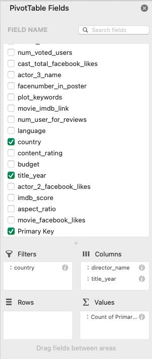
Attached are pics of the pivot table fields and all the headers/categories.

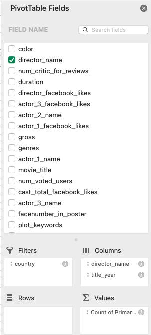
PivotTable Fields FIELD NAME Search fields ООООООООООООООО color director_name num_critic_for_reviews duration director_faceb PivotTable Fields FIELD NAME Q Search fields OOOOOOOOOOOOOOOOO num_voted_users cast_total_facebook_likes actor_3_name facenum

PivotTable Fields FIELD NAME 0 0 0 0 0 0 0 0 0 000 000 color director_name num_critic_for_reviews duration director_facebook_likes actor_3 facebook_likes actor_2_name actor_1_facebook_likes gross genres Q Search fields: actor_1_name movie title num_voted_users cast_total facebook_likes actor_3_name facenumber_in_poster plot keywords Filters : country E Rows III Columns : director_name : title_year values : Count of Primar...

Step by Step Solution

There are 3 Steps involved in it

1 Expert Approved Answer

Step: 1 Unlock

Since I cannot view attached images Ill provide you with instructions on how to create the pivot tab... View full answer

Question Has Been Solved by an Expert!

Get step-by-step solutions from verified subject matter experts

Step: 2 Unlock

Step: 3 Unlock

Students Have Also Explored These Related Accounting Questions!

Apples stated strategy for each of these years and analyze each Apple ratio from one year to the next during this time period. Be sure to explain what the ratio indicates in general, as well as with...

Give systematic IUPAC names for each of the following: (a) (b) (c) (d) (e) (f) (g) (h) Br Br Cl

Give names for each of the following bicyclic alkanes: (a) (b) (c) (d) (e) (f) Write the structure of a bicyclic compound that is a constitutional isomer of bicyclo[2.2.0]hexane and give its name. CI...

In the last chapter, you modified some tables for Roseys Roses. Now the company would like you to help it create some queries to extract information from the database. Make the following changes...

Harold and Helen Nash are saving for the college education of their newborn daughter, Susan. The Nashes estimate that college expenses will run $30,000 per year when their daughter reaches college in...

2. The project has received the go-ahead and you now face the reality of mobilizing your team and starting work in a foreign country. What special project challenges can you expect, and how will you...

In Integrative Case 10.1, we projected financial statements for Starbucks for Years +1 through +5. In this portion of the Starbucks Integrative Case, we use the projected financial statements from...

A firm is considering purchasing equipment to manufacture a new product. The equipment will cost $3M, and expected net cash inflows are $0.35M indefinitely. If market demand for the product is low,...

Lufthansa Group operates an international airline based in Germany. Lufthansa files its annual reports under International Financial Reporting Standards (IFRS). In its 2012 Annual Report to...

The P04_03.xlsx file contains four tables on four separate sheets with information about a companys sales in the latter part of 2018. These tables are not currently related, but they are relatable...

14.14 By some estimates, as many as one-fourth of the LBOs between 1987 and 1990 (the first mega-LBO boom) went bankrupt. The data in Table 14.6 illustrate the extent of the leverage associated with...

3. Construct the shear force and bending moment diagrams for the beam shown below. 20 kips 12 kips 1.5 kips/ft B C E D 6ft 8 ft 10 ft- -8 ft-

home seeker lindsay wants to increase her credit score so she can qualify for a conventional loan at a lower interest rate. To do this, Lindsay needs to focus on several factors that go into...

Most married couples view the early years of marriage as O deeply satisfying O the most stressful period of their relationship O a "trial period," to see if they want to stay together confusing, and...

A bank sells a "three against six" $3,000,000 FRA for a three-month period beginning three months from today and ending six months from today. The purpose of the FRA is to cover the interest rate...

Early Historical Development of Applied Behavior Analysis In 1913, John B. Watson was the first American psychologist to call himself a "behaviorist." From 1913 to 1974, a series of events and...

Which of the following is not a category in the Net Promoter Score methodology?

2.) Find the Laplace transform of f(t) 7e-St cos 2t +9 sinh2 2t. Use Laplace Table. %3D

CVP analysis, service firm Wildlife Escapes generates average revenue of $4,000 per person on its five-day package tours to wildlife parks in Kenya. The variable costs per person are: Annual fixed...

Standard-costing with beginning and ending work in process. Paquitas Pearls Company (PPC) is a manufacturer of knock off jewelry. Paquita attends Fashion Week in New York City every September and...

Target pricing, target cost, and value engineering. Avery, Inc., manufactures component parts. One product, TX40, has annual sales of 50,000 units. Avery sells TX40 for $40.60 per unit. Avery has two...

Consider the following balance sheet for DEF Partnership: Suppose Daniel wishes to exit the partnership completely. After discussions with Edward and Frances, the partners agree to let Daniel choose...

Jorgensen High Tech Inc. is a calendar-year, accrual-method taxpayer. At the end of year 1, Jorgensen accrued and deducted the following bonuses for certain employees for financial accounting...

Cara, Bob, and Steve want to begin a business on January 1, 2016. The individuals are considering three business formsC corporation, partnership, and S corporation. Cara has investment land with a...