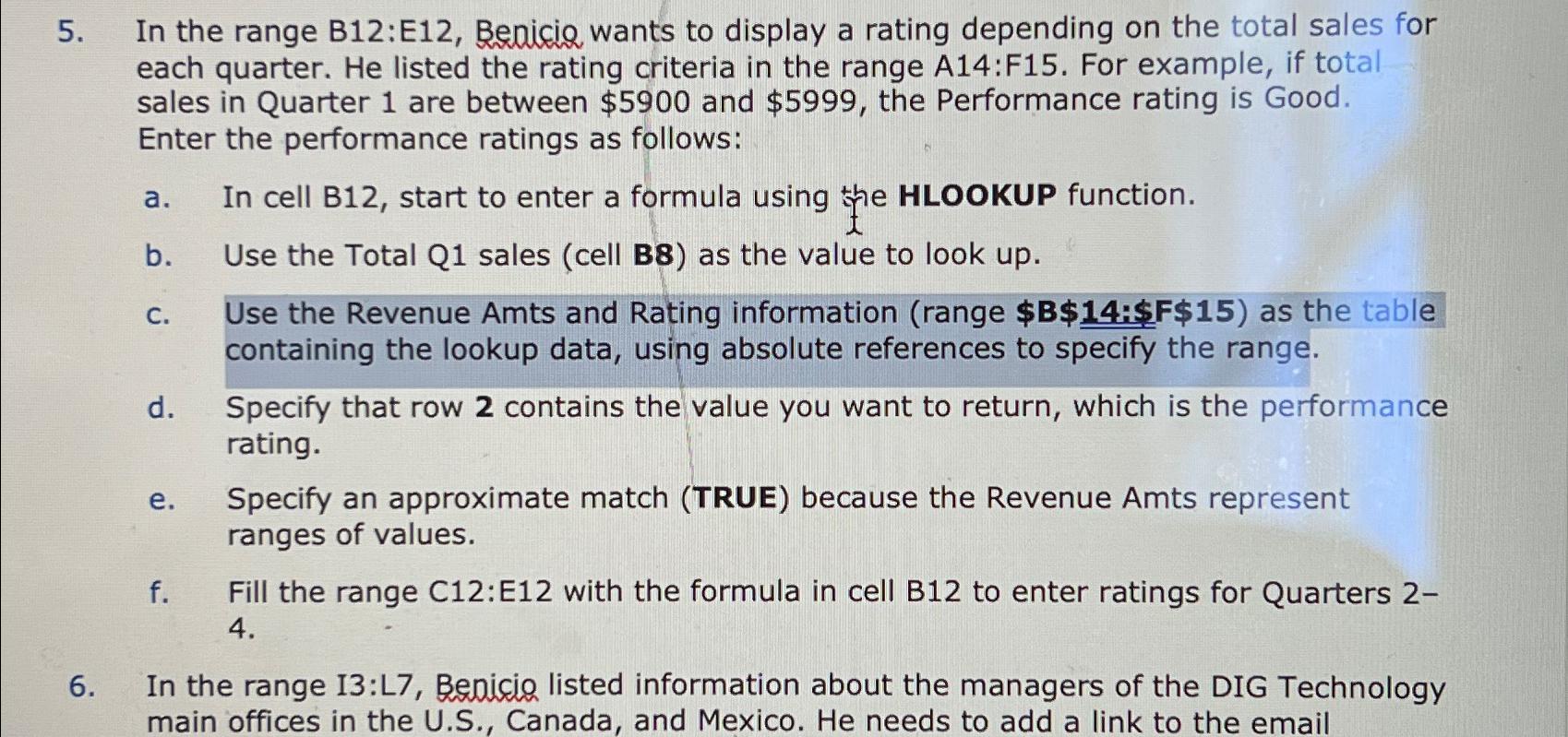
In the range $B12$:$E12,$ Bepicio wants to display a rating depending on the total sales for each quarter. He listed the rating criteria in the range A$14$:F$15.$ For example, if total sales in Quarter $1$ are between $$5900$ and $$5999,$ the Performance rating is Good. Enter the performance ratings as follows:

a$.$ In cell B$12,$ start to enter a formula using the HLOOKUP function.

b$.$ Use the Total Q$1$ sales $($cell B$8)$ as the value to look up$.$

c$.$ Use the Revenue Amts and Rating information $($range $$BB14$:$F $$15)$ as the table containing the lookup data, using absolute references to specify the range.

d$.$ Specify that row $2$ contains the value you want to return, which is the performance rating.

e$.$ Specify an approximate match $($TRUE$)$ because the Revenue Amts represent ranges of values.

f$.$ Fill the range C$12$:E$12$ with the formula in cell B$12$ to enter ratings for Quarters $24.$

In the range $I3$:$L7,$ Benicio listed information about the managers of the DIG Technology main offices in the U$.$S$.,$ Canada, and Mexico. He needs to add a link to the email