In this exercise we compute and simulate the push$-$forward map T that transforms a reference density r into a

target density p$.$ Recall that the quantile function of a $($univariate$)$ random variable X is defined as the inverse of

its cumulative distribution function $($cdf$)$ F:

F$($x$)=$ Pr$($X x$),$ Q$($u$)=$ F

$1$

$($u$),$ u in $(0,1).(1)$

We assume F is continuous and strictly increasing so that Q$1=$ F$.$ A nice property of the quantile function,

relevant to sampling, is that if U $$ Uniform$(0,1),$ then Q$($U$)$ F$.$

In the following, do not confuse cdf $($signaled by uppercase letters$)$ with pdf $($i$.$e$.,$ density, signaled by lowercase

letters$).$

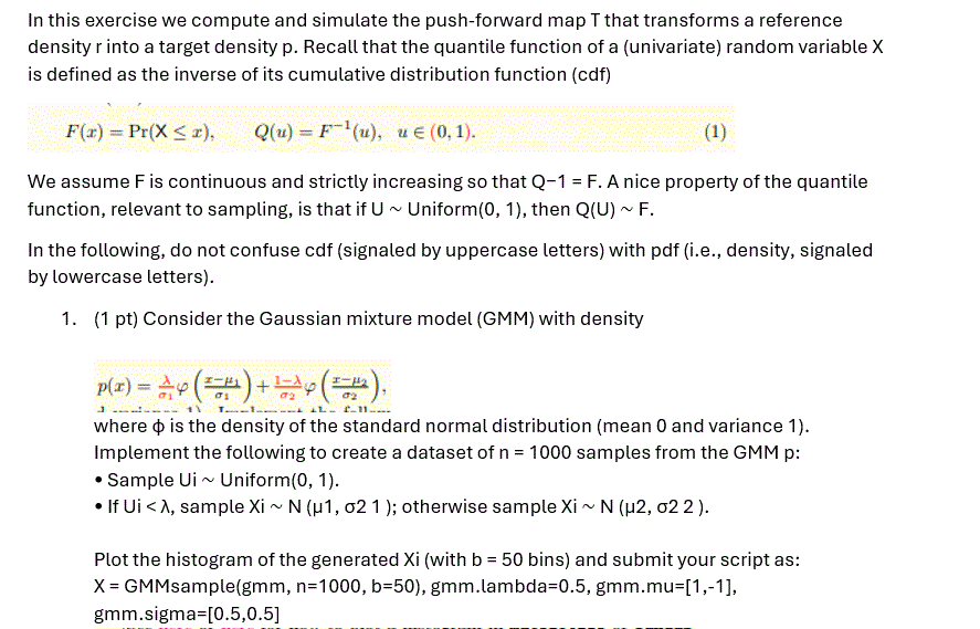
$1.(1$ pt$)$ Consider the Gaussian mixture model $($GMM$)$ with density p$($x$)=\backslash$lambda

$\backslash$sigma $1$

$\backslash$phi

x$1$

$\backslash$sigma $1$

$+$

$1\backslash$lambda

$\backslash$sigma $2$

$\backslash$phi

x$2$

$\backslash$sigma $2$

$,$ where

$\backslash$phi is the density of the standard normal distribution $($mean $0$ and variance $1).$ Implement the following to

create a dataset of n $=1000$ samples from the GMM p:

$$ Sample Ui $$ Uniform$(0,1).$

$$ If Ui $<mtext\; id="EditorElement\_7921930"></mtext><mi\; id="EditorElement\_7921931">\backslash </mi>$lambda $,$ sample Xi $$ N $(1,\backslash$sigma $2$

$1$

$)$; otherwise sample Xi $$ N $(2,\backslash$sigma $2$

$2$

$).$

Plot the histogram of the generated Xi $($with b $=50$ bins$)$ and submit your script as

X $=$ GMMsample$($gmm$,$ n$=1000,$ b$=50),$ gmm$.$lambda$=0\mathrm{.}5,$ gmm$.$mu$=[1,-1],$ gmm$.$sigma$=[0\mathrm{.}5,0\mathrm{.}5]$

$[$See here or here for how to plot a histogram in matplotlib or pandas $($or numpy if you insist$).]$

Ans: A

$2.(2$ pts$)$ Compute Ui $=\backslash$Phi $1$

F$($Xi$)),$ where F is the cdf of the GMM in Ex $2\mathrm{.}1$ and $\backslash$Phi is the cdf of standard

normal. Plot the histogram of the generated Ui $($with b bins$).$ From your inspection, what distribution should

Ui follow $($approximately$)?$ Submit your script as GMMinv$($X$,$ gmm$,$ b$=50).$

$[$This page may be helpful.$]$

Ans: A

$3.(2$ pts$)$ Let Z $$ N $(0,1).$ We now compute the push$-$forward map T so that T$($Z$)=$ X $$ p $($the GMM in Ex

$2\mathrm{.}1).$ We use the formula:

T$($z$)=$ Q$(\backslash$Phi $($z$)),(2)$

where $\backslash$Phi is the cdf of the standard normal distribution and Q $=$ F

$1$

is the quantile function of X$,$

namely the GMM p in Ex $2\mathrm{.}1.$ Implement the following binary search Algorithm $1$ to numerically

compute T$.$ Plot the function T with input z in $[5,5]($increment $0\mathrm{.}1).$ Submit your main script as

BinarySearch$($F$,$ u$,$ lb$=-100,$ ub$=100,$ maxiter$=100,$ tol$=1$e$-5),$ where F is a function. You may need

to write another script to compute and plot T $($based on BinarySearch$).$

Algorithm $1$: Binary search for solving a monotonic nonlinear equation F$($x$)=$ u$.$

Input: u in $(0,1),$ lb ub$,$ maxiter, tol

Output: x such that $|$F$($x$)$ u tol

$1$ while F$($lb$)>$ u do $//$ lower bound too large

$2$ ub $$ lb

$3$ lb $2$ lb

$4$ while F$($ub$)$ u do $//$ upper bound too small

$5$ lb $$ ub

$6$ ub $2$ ub

$7$ for i $=1,...,$ maxiter do

$8$ x $$ lb$+$ub

$2$

$//$ try middle point

$9$ t $$ F$($x$)$

$10$ if t $>$ u then

$11$ ub $$ x

$12$ else

$13$ lb $$ x

$14$ if $|$t $$ u tol then

$15$ break

Ans: A

$4.(2$ pts$)$ Sample $($independently$)$ Zi $$ N $(0,1),$ i $=1,...,$ n $=1000$ and let X$$

i $=$ T$($Zi$),$ where T is computed

by your BinarySearch. Plot the histogram of the generated X$$

i $($with b bins$)$ and submit your script as

PushForward$($Z$,$ gmm$).$ Is the histogram similar to the one in Ex $2\mathrm{.}1?$

Ans: A

$5.(1$ pt$)$ Now let us compute U$$

i $=\backslash$Phi $1$

F$($X$$

i$))$ as in Ex $2\mathrm{.}2,$ with X$$

i

$$s being generated in Ex $2\mathrm{.}4.$ Plot

the histogram of the resulting U$$

i $($with b bins$).$ From your inspection what distribution should U$$

i follow

$($approximately$)?[$No need to submit any script, as you can recycle GMMinv.$]$

Ans: A