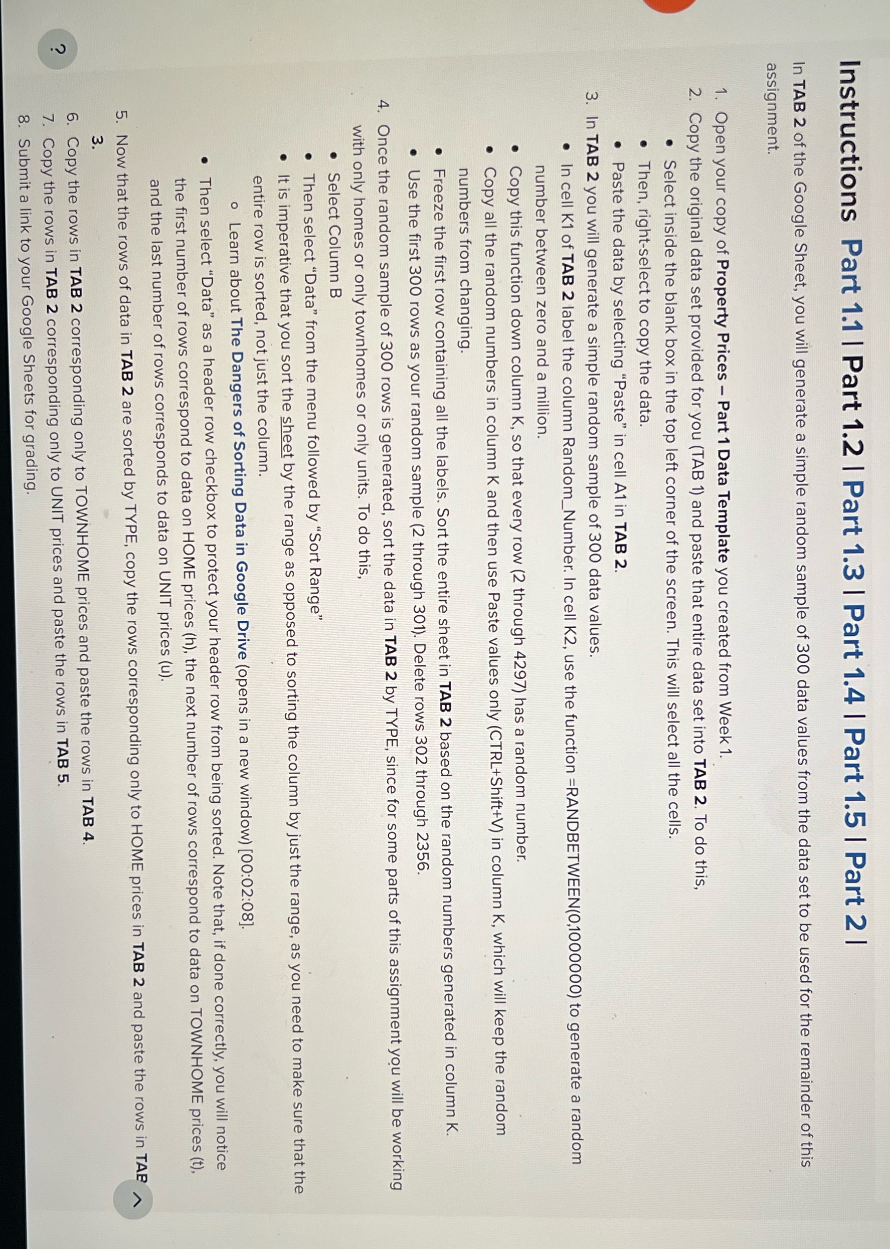
Question: Instructions Part 11| Part1.2 | Part1.3 | Part 1.4 | Part 1.5 | Part 2 | In TAB 2 of the Google Sheet, you will

Instructions Part 11| Part1.2 | Part1.3 | Part
Instructions Part 11| Part1.2 | Part1.3 | Part 1.4 | Part 1.5 | Part 2 | In TAB 2 of the Google Sheet, you will generate a simple random sample of 300 data values from the data set to be used for the remainder of this assignment. 1. Open your copy of Property Prices Part 1 Data Template you created from Week 1. 2. Copy the original data set provided for you (TAB 1) and paste that entire data set into TAB 2. To do this, e Select inside the blank box in the top left corner of the screen. This will select all the cells. e Then, right-select to copy the data. e Paste the data by selecting \"Paste\" in cell Al1in TAB 2. 3. In TAB 2 you will generate a simple random sample of 300 data values. e In cell K1 of TAB 2 label the column Random_Number. In cell K2, use the function =RANDBETWEEN(0,1000000) to generate a random number between zero and a million. e Copy this function down column K, so that every row (2 through 4297) has a random number. e Copy all the random numbers in column K and then use Paste values only (CTRL+Shift+V) in column K, which will keep th e random numbers from changing. e Freeze the first row containing all the labels. Sort the entire sheet in TAB 2 based on the random numbers generat e Use the first 300 rows as your random sample (2 through 301). Delete rows 302 through 2356. 4. Once the random sample of 300 rows is generated, sort ed in column K. the data in TAB 2 by TYPE, since for some parts of this assignment you will be working with only homes or only townhomes or only units. To do this, e Select Column B e Then select \"Data\" from the menu followed by \"Sort Range\" e |t is imperative that you sort the sheet by the range as opposed to sorting the column by just the range, as you need to make sure that the entire row is sorted, not just the column. 1 o Learn about The Dangers of Sorting Data in Google Drive (opens in a new window) [00:02:08]. e Then select \"Data\" as a header row checkbox to protect your header row from being sorted. Note that, if done correctly, you will notice the first number of rows correspond to data on HOME prices (h), the next number of rows correspond to data on TOWNHOME prices (t), and the last number of rows corresponds to data on UNIT prices (u). 5. Now that the rows of data in TAB 2 are sorted by TYPE, copy the rows corresponding only to HOME prices in TAB 2 and paste the rows in TAB A S s 6. Copy the rows in TAB 2 corresponding only to TOWNHOME prices and paste the rows in TAB 4. e 7. Copy the rows in TAB 2 corresponding only to UNIT prices and paste the rows in 4>.w 5 2. Submit a link to your Google Sheets for grading

Step by Step Solution

There are 3 Steps involved in it

1 Expert Approved Answer
Step: 1 Unlock blur-text-image
Question Has Been Solved by an Expert!

Get step-by-step solutions from verified subject matter experts

Step: 2 Unlock
Step: 3 Unlock

Students Have Also Explored These Related Human Resource Management Questions!