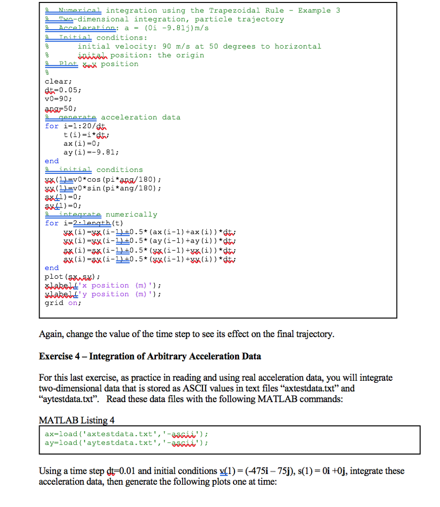
Question: integration using the Trapezoidal Rule-Example 3 -dimensional integration, particle trajectory Acceleration: a(0i 9.81j)m/s conditions: initial velocity: 90 m/s at 50 degrees to horizontal ivtat position:


integration using the Trapezoidal Rule-Example 3 -dimensional integration, particle trajectory Acceleration: a(0i 9.81j)m/s conditions: initial velocity: 90 m/s at 50 degrees to horizontal ivtat position: the origin plat position clear dt-0.05; v0-90; enerate acceleration data for i-l:20/dt ax (i)-0 ay (i)9.81; end conditions vxvO*cos (pi*apa/180); x(1v0*sin (pi*ang/180) 831) 0; e numerically for i-2 ength(t) )-vx(i-110.5* (ay(i-1) +ay (i)) dt end plot (sxArSH); xlabel'x position (m) ) vlabei'y position (m)) grid on; Again, change the value of the time step to see its effect on the final trajectory Exercise 4 - Integration of Arbitrary Acceleration Data For this last exercise, as practice in reading and using real acceleration data, you will integrate two-dimensional data that is stored as ASCII values in text files axtestdata.txt" and "aytestdata.txt". Read these data files with the following MATLAB commands MATLAB Listing 4 ax-load ('axtestdata.txt',"-asii'); ay-load ('aytestdata.txt',-saii) Using a time step dt 0.01 and initial conditions v(1)-(-475i-75j), s(1) 0i +0j, integrate these acceleration data, then generate the following plots one at time integration using the Trapezoidal Rule-Example 3 -dimensional integration, particle trajectory Acceleration: a(0i 9.81j)m/s conditions: initial velocity: 90 m/s at 50 degrees to horizontal ivtat position: the origin plat position clear dt-0.05; v0-90; enerate acceleration data for i-l:20/dt ax (i)-0 ay (i)9.81; end conditions vxvO*cos (pi*apa/180); x(1v0*sin (pi*ang/180) 831) 0; e numerically for i-2 ength(t) )-vx(i-110.5* (ay(i-1) +ay (i)) dt end plot (sxArSH); xlabel'x position (m) ) vlabei'y position (m)) grid on; Again, change the value of the time step to see its effect on the final trajectory Exercise 4 - Integration of Arbitrary Acceleration Data For this last exercise, as practice in reading and using real acceleration data, you will integrate two-dimensional data that is stored as ASCII values in text files axtestdata.txt" and "aytestdata.txt". Read these data files with the following MATLAB commands MATLAB Listing 4 ax-load ('axtestdata.txt',"-asii'); ay-load ('aytestdata.txt',-saii) Using a time step dt 0.01 and initial conditions v(1)-(-475i-75j), s(1) 0i +0j, integrate these acceleration data, then generate the following plots one at time
Step by Step Solution
There are 3 Steps involved in it

Get step-by-step solutions from verified subject matter experts


