Introduction

The Conditional Formatting tool in Microsoft Excel is designed to give you and your audience quick insights into characteristics of your data. The word "conditional" indicates a rule or criterion such as: Top $10\%,$ Below Average, High$/$Medium$/$Low$,$ etc. The "formatting" indicates ways in which you can perform actions such as changing the color of the cell and$/$or text, use color bars, or icons. The result is that viewers can gain insights into the data very quickly without having to examine each individual data value.

To perform Conditional Formatting, you first select the cells to which you would like to apply the formatting. Then select the Conditional Formatting tool which is in the Home tab in Excel and Excel Online. From there, you will find all the different conditions and formats you can apply to the data you selected.

In the spreadsheet below you find columns containing the same data. Above each column is a conditional formatting rule you should apply and then answer the questions relating to that task.

A note about colors and color blindness. According to the English website colourblindawareness.org:

"Colour $($color$)$ blindness $($colour vision deficiency, or CVD$)$ affects approximately $1$ in $12$ men $(8\%)$ and $1$ in $200$ women in the world. In Britain this means that there are approximately $3$ million colour blind people $($about $4\mathrm{.}5\%$ of the entire population$),$ most of whom are male. Worldwide, there are approximately $300$ million people with colour blindness, almost the same number of people as the entire population of the USA! $...$ The most common form of colour blindness is known as 'red$/$green colour blindness' and most colour blind people have one type of this."

Therefore, it is not recommended to use red and green together to make comparisons, which unfortunately, Excel does quite often by default.

The data has been collected in the Microsoft Excel Online file below. Open the spreadsheet and perform the required analysis to answer the questions below.

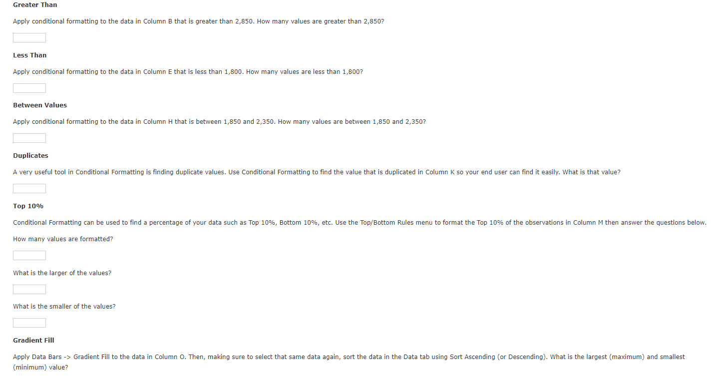
Greater Than

Apply conditional formatting to the data in Column B that is greater than $2,850.$ How many values are greater than $2,850?$

Less Than

Apply conditional formatting to the data in Column E that is less than $1,800.$ How many values are less than $1,800?$

Between Values

Apply conditional formatting to the data in Column H that is between $1,850$ and $2,350.$ How many values are between $1,850$ and $2,350?$

Duplicates

Top $10\backslash \%$

How many values are formatted?

What is the larger of the values?

What is the smaller of the values?

Gradient Fill $($minimum$)$ value? Gradient Fill

Apply Data Bars $->$ Gradient Fill to the data in Column $0.$ Then, making sure to select that same data again, sort the data in the Data tab using Sort Ascending $($or Descending$).$ What is the largest $($maximum$)$ and smallest $($minimum$)$ value?

Maximum:

Minimum:

Color Scale

Apply Color Scales to the data in Column Q$.$ Do NOT sort the data. At what position $(1$ being the top and $20$ being the bottom$)$ does the minimum data value occur?