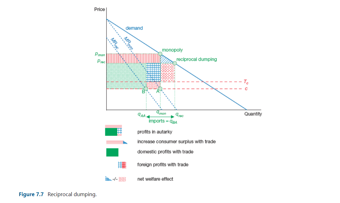
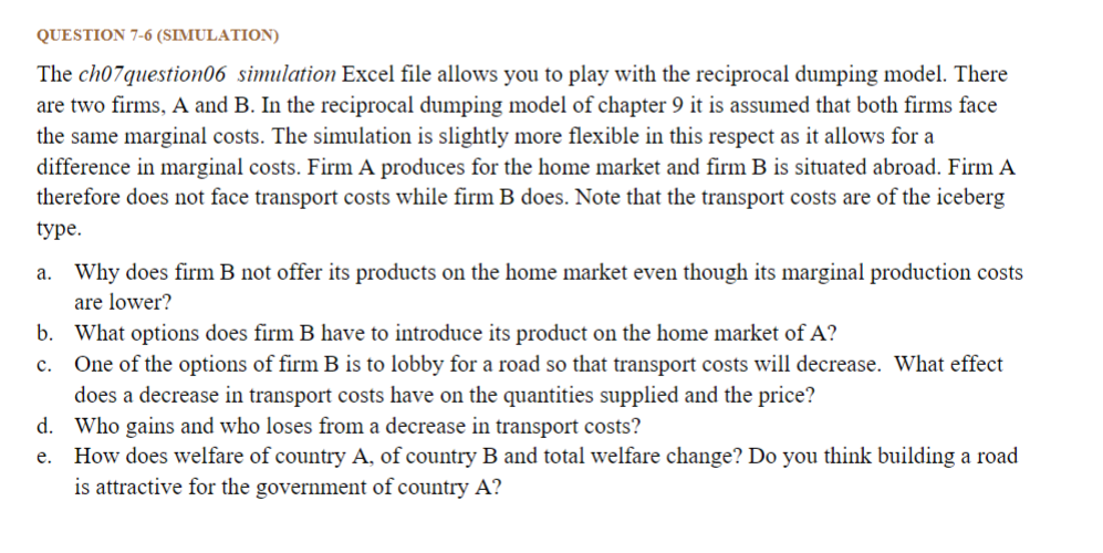
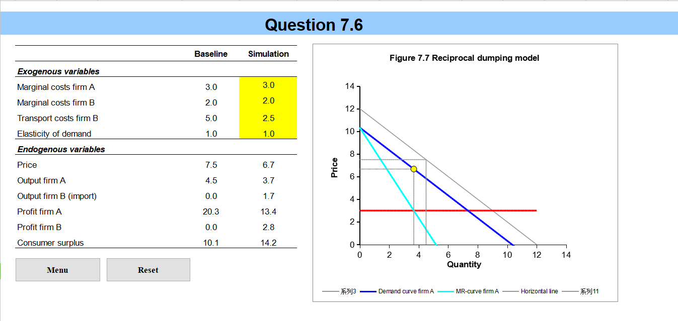
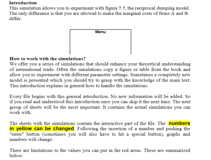
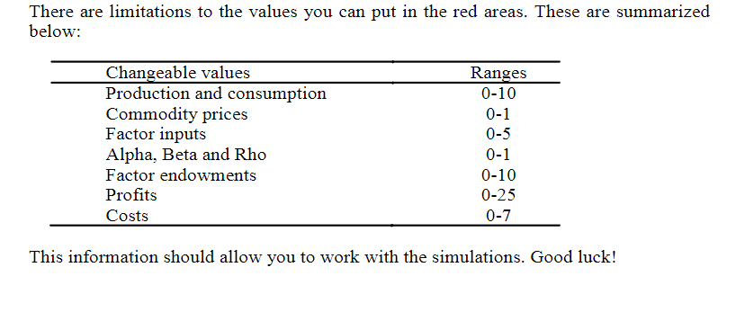
Introduction This simulation allows you to experiment with gure 7.7. the reciprocal dumping model. The only difference is that you are allowed to make the marginal costs of rms A and B differ. Menu How to work with the simulations? 1We offer you a series of simulations that should enhance your theoretical understanding of international trade. Often the simulations copy a gure or table from the book and allow you to experiment with different parameter settings. Sometimes a completely new model is presented which you should try to grasp with the knowledge of the main text. This introduction explains in general how to handle the simulations. Every file begins with this general introduction. No new information will be added. So if you read and understood this introduction once you can skip it the next time. The next group of sheets will be the most important. It contains the actual simulations you can work with. The sheets with the simulations contain the interactive part of the le. The numbers in yellow can be changed. Following the insertion of a number and pushing the "enter" button {sometimes you will also have to hit a special button)= graphs and numbers will change. There are limitations to the values you can put in the red areas. These are summarized below: There are limitations to the values you can put in the red areas. These are summarized below: Changeable values Ranges Production and consumption 0-10 Commodity prices 0 -1 Factor inputs 0 -5 Alpha, Beta and Rho 0-1 Factor endowments 0-10 Prots 0-2 5 Co sts 0 -7 This information should allow you to work with the simulations. Good luck! Price demand .".......... MRrec monopoly Pmon Prec reciprocal dumping To C B 9AA4 9mon 9rec Quantity imports = 9BA profits in autarky increase consumer surplus with trade domestic profits with trade foreign profits with trade net welfare effect Figure 7.7 Reciprocal dumping.QUESTION 7-6 (SIMULATION) The ch07question06 simulation Excel file allows you to play with the reciprocal dumping model. There are two firms, A and B. In the reciprocal dumping model of chapter 9 it is assumed that both firms face the same marginal costs. The simulation is slightly more flexible in this respect as it allows for a difference in marginal costs. Firm A produces for the home market and firm B is situated abroad. Firm A therefore does not face transport costs while firm B does. Note that the transport costs are of the iceberg type. a. Why does firm B not offer its products on the home market even though its marginal production costs are lower? b. What options does firm B have to introduce its product on the home market of A? c. One of the options of firm B is to lobby for a road so that transport costs will decrease. What effect does a decrease in transport costs have on the quantities supplied and the price? d. Who gains and who loses from a decrease in transport costs? e. How does welfare of country A, of country B and total welfare change? Do you think building a road is attractive for the government of country A?Question 7.6 Baseline Simulation Figure 7.7 Reciprocal dumping model Exogenous variables Marginal costs firm A 3.0 3.0 14- Marginal costs firm B 2.0 2.0 12- Transport costs firm B 5.0 2.5 Elasticity of demand 1.0 1.0 10 - Endogenous variables 8 Price 7.5 6.7 Price Output firm A 4.5 3.7 6 . Output firm B (import) 0.0 1.7 4 Profit firm A 20.3 13.4 Profit firm B 0.0 2.8 2 Consumer surplus 10.1 14.2 0 2 4 6 8 10 12 14 Menu Reset Quantity :513 - Demand curve firm A - MR-curve firm A Horizontal line 51 11