

Intuitively, we can think of an option's value as C=E[Cr]e i.e., the option's expected payoff E[C]...
Fantastic news! We've Found the answer you've been seeking!
Question:
![Intuitively, we can think of an option's value as C=E[Cr]e i.e., the option's expected payoff E[C] discounted](https://dsd5zvtm8ll6.cloudfront.net/si.experts.images/questions/2023/09/6513d14a0e466_1695797574734.jpg)

Transcribed Image Text:
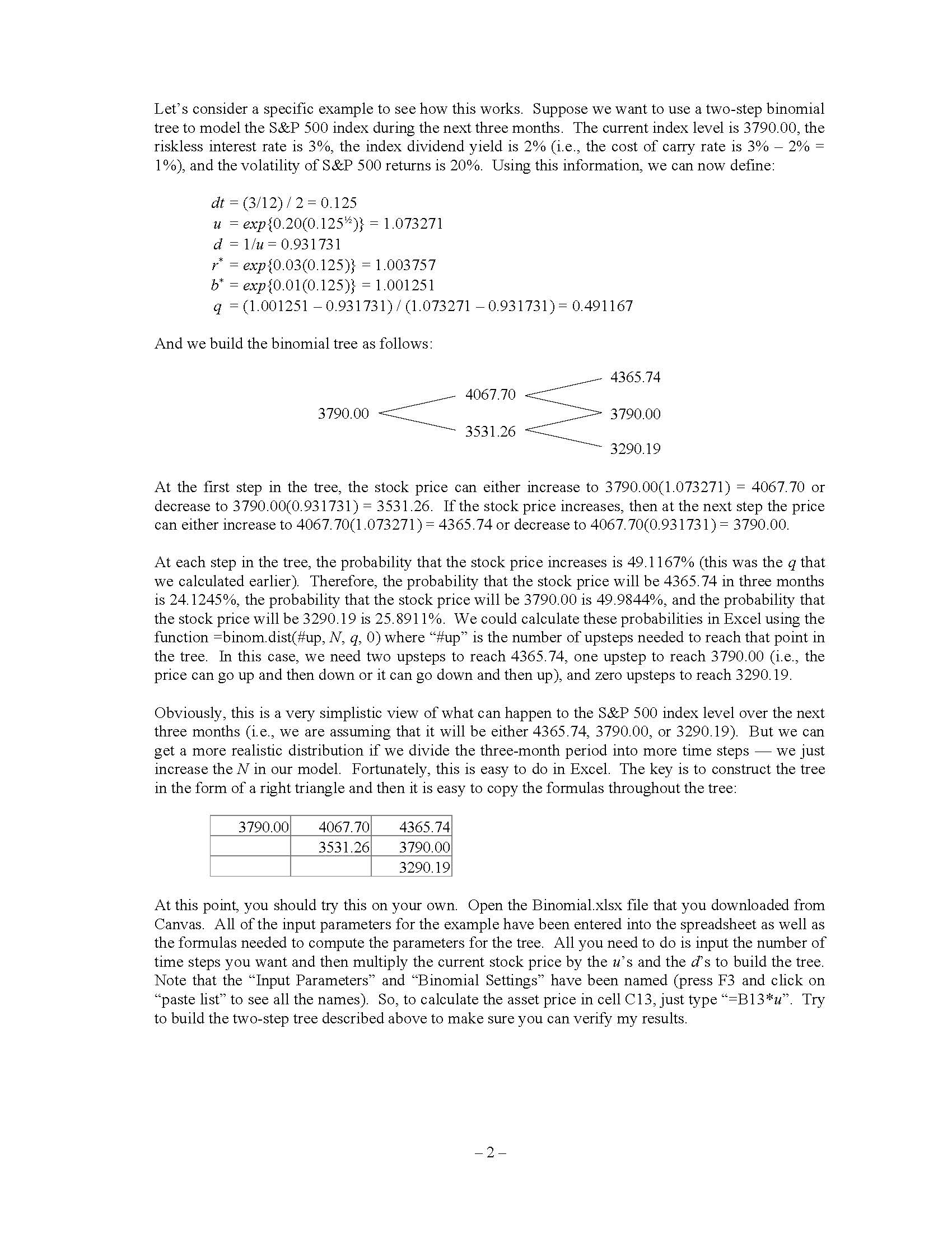
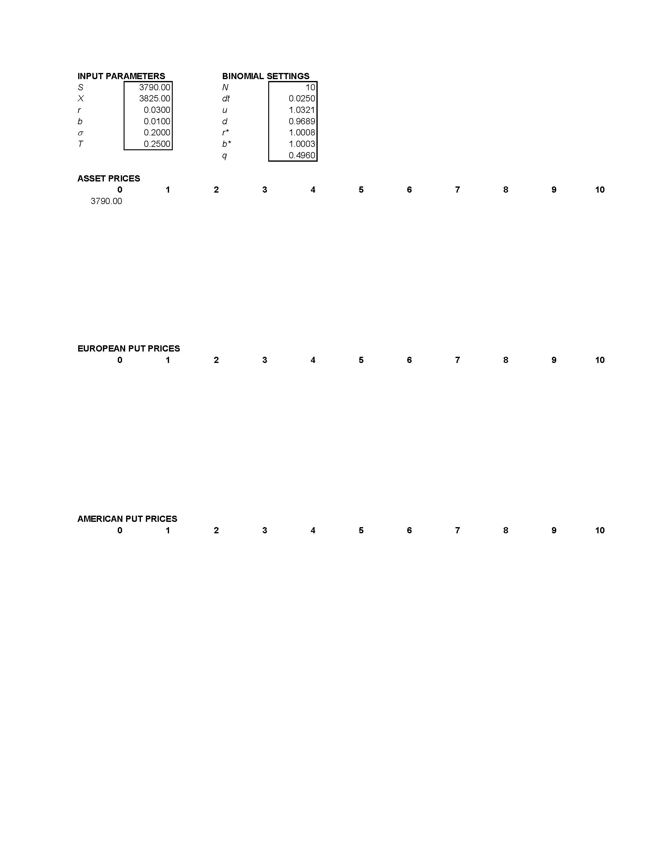
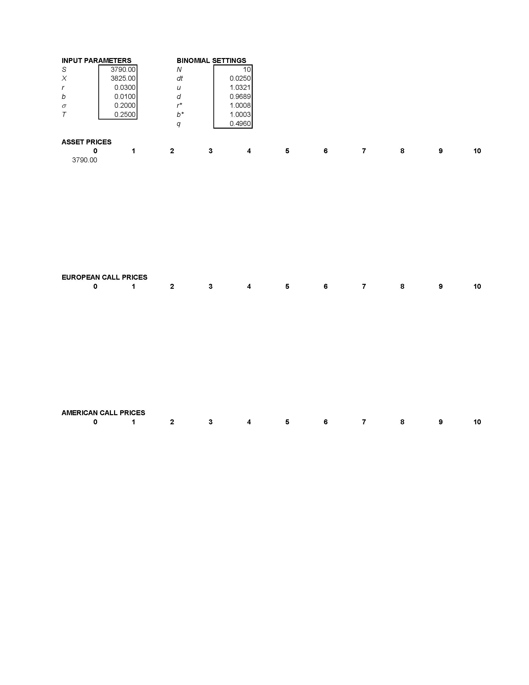
Intuitively, we can think of an option's value as C=E[Cr]e¹¹ i.e., the option's expected payoff E[C] discounted back by the option's required rate of return (rc). To implement this equation, we need to address two issues: 1) how do we compute the option's expected payoff, and 2) what is the option's required rate of return? The purpose of this assignment is to get you thinking about the first of these issues. An option's expected payoff depends on the distribution of possible asset prices at the time the option expires. For example, consider a two-month call option on a stock. Suppose the current stock price is $50 and the option's exercise price is $60. If there is no chance that the stock price will be greater than $60 in two months, then the option's expected payoff is zero. On the other hand, if the probability of realizing a stock price greater than $60 is large, then the option's expected payoff is large. In order to model the distribution of stock prices at expiration, we will use the following approach. (Warning: don't spend too much time studying the details until we get to the example that follows.) $ u²S S d's The time from now until the option's expiration is T. We divide this time period into N time steps so that the length of each time step is dt = T/N. We assume that the asset price follows a binomial process which means that at each time step the asset price either increases or decreases. If the price increases, the return is u = explo(dt)"} where o is the annualized volatility of the asset's returns. And if the price decreases, the return is d-1/u. We will assume that the probability that the asset price increases at each step is q-(b* -d)/(u-d) where be is the asset's cost of carry rate per time step, and we will define * = e(*) as the riskless interest rate per time step. Let's consider a specific example to see how this works. Suppose we want to use a two-step binomial tree to model the S&P 500 index during the next three months. The current index level is 3790.00, the riskless interest rate is 3%, the index dividend yield is 2% (i.e., the cost of carry rate is 3% - 2% = 1%), and the volatility of S&P 500 returns is 20%. Using this information, we can now define: dt = (3/12)/2 = 0.125 U d r* = exp{0.03(0.125)} = 1.003757 b* = exp{0.01(0.125)} = 1.001251 q = (1.001251 -0.931731)/(1.073271 -0.931731) = 0.491167 exp{0.20(0.125¹)} = 1.073271 1/u 0.931731 = And we build the binomial tree as follows: 3790.00 3790.00 4067.70 3531.26 4067.70 3531.26 At the first step in the tree, the stock price can either increase to 3790.00(1.073271) = 4067.70 or decrease to 3790.00(0.931731) = 3531.26. If the stock price increases, then at the next step the price can either increase to 4067.70(1.073271) = 4365.74 or decrease to 4067.70(0.931731) = 3790.00. 4365.74 3790.00 3290.19 4365.74 At each step in the tree, the probability that the stock price increases is 49.1167% (this was the 9 that we calculated earlier). Therefore, the probability that the stock price will be 4365.74 in three months is 24.1245%, the probability that the stock price will be 3790.00 is 49.9844%, and the probability that the stock price will be 3290.19 is 25.8911%. We could calculate these probabilities in Excel using the function =binom.dist(#up, N, q, 0) where "#up" is the number of upsteps needed to reach that point in the tree. In this case, we need two upsteps to reach 4365.74, one upstep to reach 3790.00 (i.e., the price can go up and then down or it can go down and then up), and zero upsteps to reach 3290.19. 3790.00 Obviously, this is a very simplistic view of what can happen to the S&P 500 index level over the next three months (i.e., we are assuming that it will be either 4365.74, 3790.00, or 3290.19). But we can get a more realistic distribution if we divide the three-month period into more time steps we just increase the N in our model. Fortunately, this is easy to do in Excel. The key is to construct the tree in the form of a right triangle and then it is easy to copy the formulas throughout the tree: 3290.19 - 2- At this point, you should try this on your own. Open the Binomial.xlsx file that you downloaded from Canvas. All of the input parameters for the example have been entered into the spreadsheet as well as the formulas needed to compute the parameters for the tree. All you need to do is input the number of time steps you want and then multiply the current stock price by the u's and the d's to build the tree. Note that the "Input Parameters" and "Binomial Settings" have been named (press F3 and click on "paste list" to see all the names). So, to calculate the asset price in cell C13, just type "=B13*u". Try to build the two-step tree described above to make sure you can verify my results. The Assignment Build a 10-step binomial tree to model the S&P 500 index during the next three months. The current index level is 3790.00, the riskless interest rate is 3%, the index dividend yield is 2% and the index volatility rate is 20%. You can start with the same spreadsheet as before but remember to change the N under the columns labeled "Binomial Settings." When you are finished with the tree, you should have 11 possible asset prices at the end of the three- month period. Now, in the column next to each asset price, compute the corresponding three-month continuously compounded return, i.e., =ln(S7/So). In the next column, use the binom. dist() function described above to compute the probability of realizing each of these returns. You might want to add up the probabilities to make sure that they sum to one. Use your completed tree to answer the following questions: 1. Compute the expected three-month continuously compounded return. To do this, multiply each of the returns (i.e., =ln(S7/So)) by their corresponding probabilities and then add them all up. 2. Compute the expected stock price in three months. Do this the same way as in question 1 above, except now multiply the stock prices (i.e., Sr) by the probabilities. Note: You don't need to do anything yet with the cells below row 25 (i.e., the option prices). We will complete this part of the spreadsheet after we discuss option valuation in class. The Deliverable Print your completed spreadsheet on a single page of paper. Write your name in the top corner. Write your answer for the expected three-month return (question 1 above) below your name and then below that write your answer for the expected stock price (question 2). Upload this printout to Canvas. Finally, download "BlackScholes.xlsx" from the course page in Canvas. You don't need to do any- thing with this spreadsheet; just make sure that it's on your laptop and ready to use during class. - 3- INPUT PARAMETERS S cxobt X T ASSET PRICES 0 3790.00 3790.00 3825.00 0.0300 0.0100 0.2000 0.2500 EUROPEAN PUT PRICES 1 0 AMERICAN PUT PRICES 1 0 N 2 2 BINOMIAL SETTINGS zo sot bo N dt b* 3 10 0.0250 1.0321 0.9689 1.0008 1.0003 0.4960 4 4 LO 5 LO 5 LO (o (0) (0) 7 7 7 00 8 8 9 9 10 10 10 INPUT PARAMETERS S cxobt X T ASSET PRICES 0 3790.00 3790.00 3825.00 0.0300 0.0100 0.2000 0.2500 EUROPEAN CALL PRICES 1 0 AMERICAN CALL PRICES 1 0 N 2 2 BINOMIAL SETTINGS zo sot bo N dt b* 3 10 0.0250 1.0321 0.9689 1.0008 1.0003 0.4960 4 4 LO 5 LO 5 LO (o (0) (0) 7 7 7 00 8 8 9 9 10 10 10 Intuitively, we can think of an option's value as C=E[Cr]e¹¹ i.e., the option's expected payoff E[C] discounted back by the option's required rate of return (rc). To implement this equation, we need to address two issues: 1) how do we compute the option's expected payoff, and 2) what is the option's required rate of return? The purpose of this assignment is to get you thinking about the first of these issues. An option's expected payoff depends on the distribution of possible asset prices at the time the option expires. For example, consider a two-month call option on a stock. Suppose the current stock price is $50 and the option's exercise price is $60. If there is no chance that the stock price will be greater than $60 in two months, then the option's expected payoff is zero. On the other hand, if the probability of realizing a stock price greater than $60 is large, then the option's expected payoff is large. In order to model the distribution of stock prices at expiration, we will use the following approach. (Warning: don't spend too much time studying the details until we get to the example that follows.) $ u²S S d's The time from now until the option's expiration is T. We divide this time period into N time steps so that the length of each time step is dt = T/N. We assume that the asset price follows a binomial process which means that at each time step the asset price either increases or decreases. If the price increases, the return is u = explo(dt)"} where o is the annualized volatility of the asset's returns. And if the price decreases, the return is d-1/u. We will assume that the probability that the asset price increases at each step is q-(b* -d)/(u-d) where be is the asset's cost of carry rate per time step, and we will define * = e(*) as the riskless interest rate per time step. Let's consider a specific example to see how this works. Suppose we want to use a two-step binomial tree to model the S&P 500 index during the next three months. The current index level is 3790.00, the riskless interest rate is 3%, the index dividend yield is 2% (i.e., the cost of carry rate is 3% - 2% = 1%), and the volatility of S&P 500 returns is 20%. Using this information, we can now define: dt = (3/12)/2 = 0.125 U d r* = exp{0.03(0.125)} = 1.003757 b* = exp{0.01(0.125)} = 1.001251 q = (1.001251 -0.931731)/(1.073271 -0.931731) = 0.491167 exp{0.20(0.125¹)} = 1.073271 1/u 0.931731 = And we build the binomial tree as follows: 3790.00 3790.00 4067.70 3531.26 4067.70 3531.26 At the first step in the tree, the stock price can either increase to 3790.00(1.073271) = 4067.70 or decrease to 3790.00(0.931731) = 3531.26. If the stock price increases, then at the next step the price can either increase to 4067.70(1.073271) = 4365.74 or decrease to 4067.70(0.931731) = 3790.00. 4365.74 3790.00 3290.19 4365.74 At each step in the tree, the probability that the stock price increases is 49.1167% (this was the 9 that we calculated earlier). Therefore, the probability that the stock price will be 4365.74 in three months is 24.1245%, the probability that the stock price will be 3790.00 is 49.9844%, and the probability that the stock price will be 3290.19 is 25.8911%. We could calculate these probabilities in Excel using the function =binom.dist(#up, N, q, 0) where "#up" is the number of upsteps needed to reach that point in the tree. In this case, we need two upsteps to reach 4365.74, one upstep to reach 3790.00 (i.e., the price can go up and then down or it can go down and then up), and zero upsteps to reach 3290.19. 3790.00 Obviously, this is a very simplistic view of what can happen to the S&P 500 index level over the next three months (i.e., we are assuming that it will be either 4365.74, 3790.00, or 3290.19). But we can get a more realistic distribution if we divide the three-month period into more time steps we just increase the N in our model. Fortunately, this is easy to do in Excel. The key is to construct the tree in the form of a right triangle and then it is easy to copy the formulas throughout the tree: 3290.19 - 2- At this point, you should try this on your own. Open the Binomial.xlsx file that you downloaded from Canvas. All of the input parameters for the example have been entered into the spreadsheet as well as the formulas needed to compute the parameters for the tree. All you need to do is input the number of time steps you want and then multiply the current stock price by the u's and the d's to build the tree. Note that the "Input Parameters" and "Binomial Settings" have been named (press F3 and click on "paste list" to see all the names). So, to calculate the asset price in cell C13, just type "=B13*u". Try to build the two-step tree described above to make sure you can verify my results. The Assignment Build a 10-step binomial tree to model the S&P 500 index during the next three months. The current index level is 3790.00, the riskless interest rate is 3%, the index dividend yield is 2% and the index volatility rate is 20%. You can start with the same spreadsheet as before but remember to change the N under the columns labeled "Binomial Settings." When you are finished with the tree, you should have 11 possible asset prices at the end of the three- month period. Now, in the column next to each asset price, compute the corresponding three-month continuously compounded return, i.e., =ln(S7/So). In the next column, use the binom. dist() function described above to compute the probability of realizing each of these returns. You might want to add up the probabilities to make sure that they sum to one. Use your completed tree to answer the following questions: 1. Compute the expected three-month continuously compounded return. To do this, multiply each of the returns (i.e., =ln(S7/So)) by their corresponding probabilities and then add them all up. 2. Compute the expected stock price in three months. Do this the same way as in question 1 above, except now multiply the stock prices (i.e., Sr) by the probabilities. Note: You don't need to do anything yet with the cells below row 25 (i.e., the option prices). We will complete this part of the spreadsheet after we discuss option valuation in class. The Deliverable Print your completed spreadsheet on a single page of paper. Write your name in the top corner. Write your answer for the expected three-month return (question 1 above) below your name and then below that write your answer for the expected stock price (question 2). Upload this printout to Canvas. Finally, download "BlackScholes.xlsx" from the course page in Canvas. You don't need to do any- thing with this spreadsheet; just make sure that it's on your laptop and ready to use during class. - 3- INPUT PARAMETERS S cxobt X T ASSET PRICES 0 3790.00 3790.00 3825.00 0.0300 0.0100 0.2000 0.2500 EUROPEAN PUT PRICES 1 0 AMERICAN PUT PRICES 1 0 N 2 2 BINOMIAL SETTINGS zo sot bo N dt b* 3 10 0.0250 1.0321 0.9689 1.0008 1.0003 0.4960 4 4 LO 5 LO 5 LO (o (0) (0) 7 7 7 00 8 8 9 9 10 10 10 INPUT PARAMETERS S cxobt X T ASSET PRICES 0 3790.00 3790.00 3825.00 0.0300 0.0100 0.2000 0.2500 EUROPEAN CALL PRICES 1 0 AMERICAN CALL PRICES 1 0 N 2 2 BINOMIAL SETTINGS zo sot bo N dt b* 3 10 0.0250 1.0321 0.9689 1.0008 1.0003 0.4960 4 4 LO 5 LO 5 LO (o (0) (0) 7 7 7 00 8 8 9 9 10 10 10
Expert Answer:
Answer rating: 100% (QA)
Sure here are the answers to your questions 1 Compute the expected threemonth continuously compounded return To do this we multiply each of the returns ie lnS by their corresponding probabilities and ... View the full answer

Related Book For 

Management Accounting Information for Decision-Making and Strategy Execution
ISBN: 978-0137024971
6th Edition
Authors: Anthony A. Atkinson, Robert S. Kaplan, Ella Mae Matsumura, S. Mark Young
Posted Date:
Students also viewed these accounting questions
-
You are in the business of transporting fresh fruits from South Africa to Angola. Critically discuss ANY FIVE (5) risks you could be exposed to in your supply chain. Provide relevant examples in your...
-
Planning is one of the most important management functions in any business. A front office managers first step in planning should involve determine the departments goals. Planning also includes...
-
KYC's stock price can go up by 15 percent every year, or down by 10 percent. Both outcomes are equally likely. The risk free rate is 5 percent, and the current stock price of KYC is 100. (a) Price a...
-
In Problems 2734, the given pattern continues. Write down the nth term of a sequence {a n } suggested by the pattern. 2 1 1 ,3,-, 5, 7 6 ....: 8
-
X-IM Bank has 14 million in assets and 23 million in liabilities and has sold 8 million in foreign currency trading. What is the net exposure for X-IM? For what type of exchange rate movement does...
-
What was Amazon Asset turn over ratio for 2021 & 2022? Provide a brief explanation and formula.
-
Contribution = (a) Fixed cost loss (b) Profit + variable cost (c) Sales fixed cost profit (d) None of the above Ans: (a)
-
A company seeking a line of credit at a bank was turned down. Among other things, the bank stated that the companys 2 to I current ratio was not adequate. Give reasons why a 2 to 1 current ratio...
-
After the success of the companys first two months, Santana Rey continues to operate Business Solutions. The November 30, 2019, unadjusted trial balance of Business Solutions (reflecting its...
-
Cash Flows Horiz Analysis Horiz Analysis Vertic Analysis Vertic Analysis from Oper Inc St Bal St Inc St Bal Sheet Ratios Requirement Prepare the cash flows from operations section of R. Ashburn...
-
Huron Company produces a commercial cleaning compound known as Zoom. The direct materials and direct labor standards for one unit of Zoom are given below. Direct materials Direct labor Standard...
-
Zephyr Minerals completed the following transactions involving machinery. Machine No. 1550 was purchased for cash on April 1, 2020, at an installed cost of $75,000. Its useful life was estimated to...
-
Kelly is a self-employed tax attorney whose practice primarily involves tax planning. During the year, she attended a three-day seminar regarding new changes to the tax law. She incurred the...
-
At a recently concluded Annual General Meeting (AGM) of a company, one of the shareholders remarked; historical financial statements are essential in corporate reporting, particularly for compliance...
-
4. In hypothesis, Mr. Ng wants to compare the solution in Q3 to other solutions in different conditions. If the following constraints are newly set in place, answer how much different is going to be...
-
3C2H6O2+7H2O= C2H4O3+11H2+O2+H2C2O4+CH2O2 Glycolic acid is produced electrochemically from ethylene glycol under alkaline conditions(NaOH). Hydrogen is produced at the cathode, and formic acid and...
-
On January 1, 2020, Flounder Company purchased the following two machines for use in its production process. Machine A: The cash price of this machine was $39,000. Related expenditures included:...
-
An environmentalist wants to determine if the median amount of potassium (mg/L) in rainwater in Lincoln County, Nebraska, is different from that in the rainwater in Clarendon County, South Carolina....
-
List three quantitative non financial measures of performance in a manufacturing organization of your choice.
-
What are the two essential financial elements needed to arrive at a target cost?
-
Make-or-buy and opportunity cost Premier Company manufactures gear model G37, which is used in several of its farm-equipment products. Annual production volume of G37 is 20,000 units. Unit costs for...
-
Jamie Lee has decided to purchase a certified, preowned vehicle. What might she expect as far as reliability and a warranty on the used car?
-
What daily spending items are amounts that might be reduced or eliminated to allow for higher savings amounts?
-
Jamie Lee is attracted to the low monthly payment advertised for a vehicle lease. She may well be able to afford a more expensive car than she originally thought. Jamie Lee really needs to think this...

Study smarter with the SolutionInn App