It is frequently the case that data from two or more sources needs to be combined into a single file. Even in the best case scenario when the data comes from the same technology there can be quite a bit of work which needs to be done to create the combined file. This exercisetakes you through a simplified Extract, Transform,Load (ETL) process. You will be taking twosets of data from Excel and combiningthem into a singlesource that can be analyzed. Right now, the two sets of data aresimilar, but have too many differences whichprevent records from being directlycompared across sets. You will need to createand implement rules that resolvethedifferences in the data. So you will be:

• Extracting the data from the original worksheet.
• Transforming the data using an Excel formula.
• Loading the data into a new worksheet that contains a single set ofcombined data.

Youll be workingwith data in the Excel workbook ETL Exercise.xlsx. It is acollection of orders, organizedby line item. Multiple rows can be associated with asingle order because you can order multiple items in a single order.

There are five worksheets in this workbook:

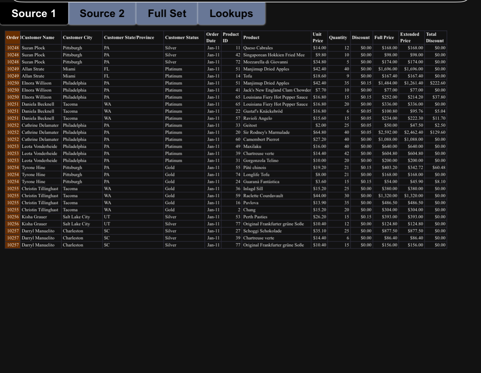
• Source 1: The first data source(29 records)
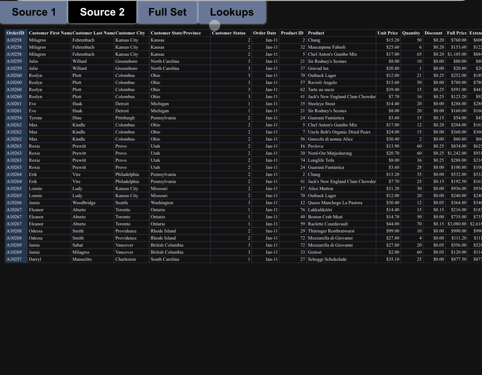
• Source 2: The second data source(32 records)
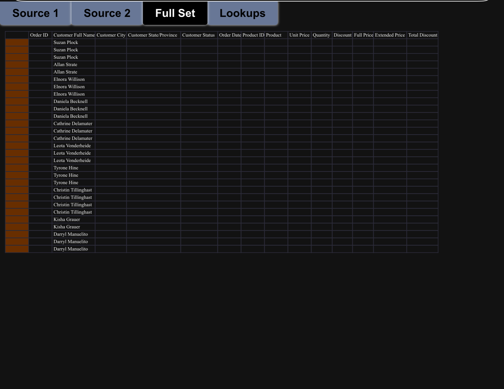
• Full Set: An empty data source that will contain a consolidated set of all59 records
• Lookups: Where wellstore the tables used to look up values. Youllusethis in Part 2.

To understand the inconsistenciesbetween the data, open the workbook and look atthe Source 1 and Source 2 worksheets. Youll notice that the data doesntquitematch up. For example, order is represented in Source1 as a fivedigit number (i.e.,10001) but in source 2 as an A followedby a five digit number (i.e., A10001).Leftas is, an analysis(such as a Pivot Table) would see this as two different orders. Thedata must be reconciled so that the format is the same.

Part 1: ETL with the OrderID field

Lets decide that the rule is to leave OrderID in Source 1 alone and removetheA from OrderID in Source 2. Try this:

1. Click on the Full Set tab.
2. Click on cell B2.
3. Press = to start a formula,switch to the Source1 tab, and click on A2there.
4. Press Enter and youllsee the OrderIDfrom Source 1.
5. Copy that formuladown to cell B30 on the Full Set tab (the section labeledData From Source 1).
6. Now click on cell B31.
7. Press = to start a formula,and type =RIGHT('Source 2'!A2,LEN('Source 2'!A2)-1) (BE CAREFUL HERE DONT FORGET THE SPACE INBETWEENSource and 2)
8. Press Enter and youllsee the OrderIDfrom Source 2 withoutthe leadingA
9. Copy that formuladown to cell B62 on the Full Set tab (the part labeledData From Source 2).

Dissecting the formula here is how we transformed the data:

• RIGHT(value,n) is an Excel function that takes the right n characters ofvalue.So RIGHT(HELLO, 2) will return LO.
• LEN(value) returns the number of characters contained in value. SoLEN(123)and LEN(DOG) both return 3.
• So LEN('Source 2'!A2)1looks at the length of the cell A2 and returnseverything exceptthe first character.Heres an example:Lets say the cellcontains A12345. The LENgthis 6, so length1 is 5. Now if you take theright 5 characters of A12345 you get only 12345.
• So youve transformed your data into a new format!

ETL with the CustomerState/Province field

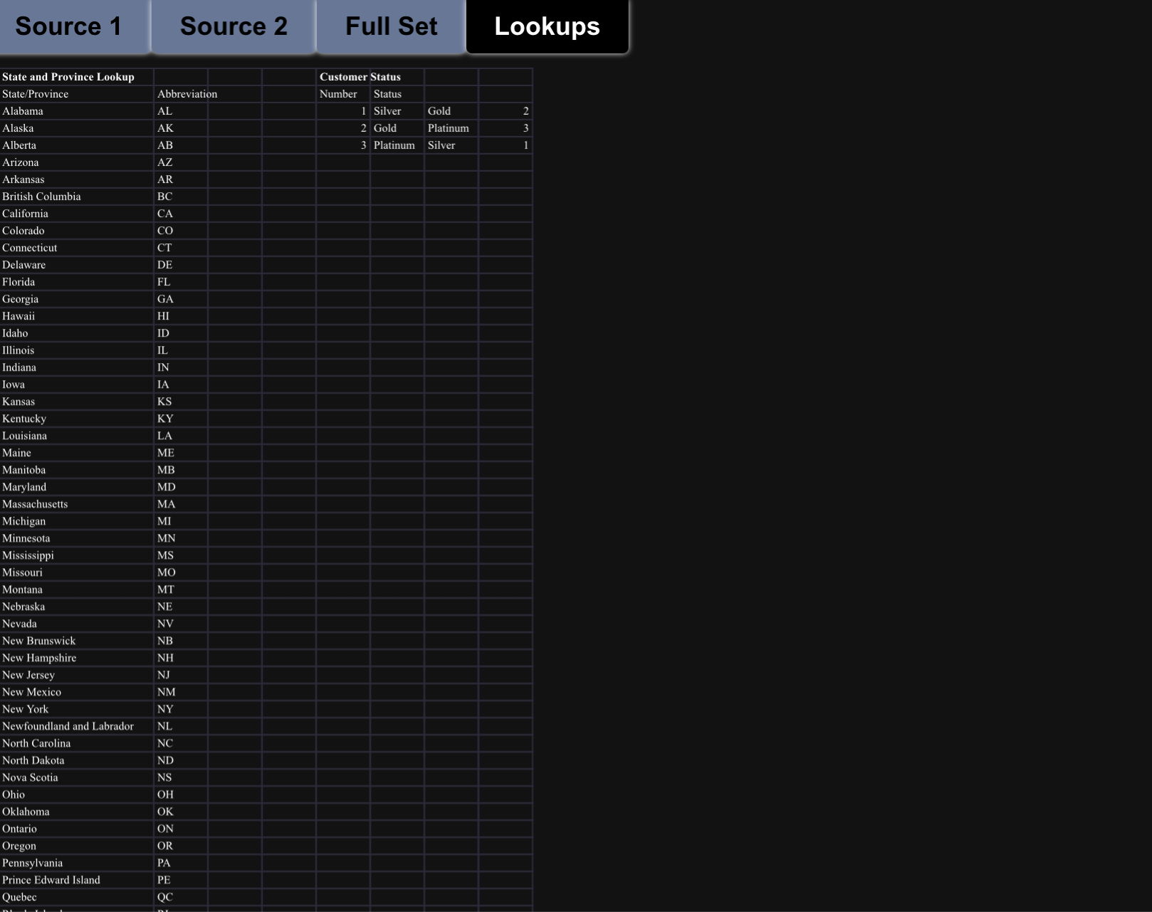
Now lets look at the Customer State/Province field. Our rule will be that state andprovinces (for Canada) names will be displayed using their abbreviation (i.e., PAinstead of Pennsylvania, ON instead of Ontario).To do this, we can use theState/Province Lookup table that has been created in the Lookups tab. Take aquick look at that table by switchingto that Lookups tab. Then followtheinstructionsbelow:

1. Click on the Full Set tab.
2. Click on cell E2.
3. Press = to start a formula,switch to the Source1 tab, and click on D2there.
4. Press Enter and youllsee the State/Province value from Source 1.
5. Copy that formuladown to cell E30 on the Full Set tab (in the sectionlabeled Data From Source 1).
6. Now click on cell E31. 7) Press = to start a formula, and type VLOOKUP('Source 2'!E2,Lookups!$A$3:$B$62,2,FALSE)

(BE CAREFUL HERE DONTFORGET THE SPACE IN BETWEENSourceand 2)

1. Press Enter and youllsee the state abbreviation from Source 2 (KS)instead of the full name (Kansas)
2. Copy that formuladown to cell E62 on the Full Set tab (in the sectionlabeled Data From Source 2).

Dissecting the formula here is how we transformed the data:

• VLOOKUP(lookup_value, table_array, column_index, range_lookup) is anExcel function that will match a value with anothervalue in a separatetable.
• So lookup_value is value that youre lookingfor. So in this case Excel willlook for the value contained in cell E2 in the Source 2 worksheet. In thiscase, that value is Kansas.
• And table_array is the table whereyoure going to do your search.Thetable is from A3 to B62 on the Lookups worksheet. Notice that the firstcolumn of that table is in alphabetical order.That is what it uses to find amatch; if the first column isnt in alphabetical order (or ascendingnumerical order) the function wont work.
• Also, you need to use the dollar signs to keep the cell references fromchanging when you copy the formula to the other cells on the Full Setworksheet. In other words, youre lookup valuekeeps changing, but yourlookuptable is always the same.
• The parameter column_index indicatescolumn number with thevaluethat is returned. Notice that column 2 has all of the stateabbreviations.
• Finally, range_lookupis TRUE if we are looking for approximatematchesand FALSE if we are looking for exact matches. Unlessyou havea good reasonto do so, always use FALSE.

Part 2: Finish the transformation process

Perform the ETL processon the rest of the fields in the Full Set worksheet:

	Customer Full Name*		Product ID		Discount
	Customer City		Product		Full Price
	Customer Status*		Unit Price		ExtendedPrice
	Order Date		Quantity		TotalDiscount*

* Theseare fields with inconsistent data between data sets Source 1 andSource 2.

In many cases youll just be copying the data from each worksheetwithouttransformation (like you did in the first five steps in Parts 1 and 2). Forexample, Order Date is represented in the same way in Source 1 and Source 2.

However, for three of the fields Customer Full Name, Customer Status, and TotalDiscount youll need to transform the data.You may transform eitherSource 1 orSource 2, depending on the transformation rule you create.

Here are a summaryof the remaining inconsistencies:

Source 1 Field	Source 2 Field
Customer Name is one field	Customer First Name and Customer LastName
	are separate fields
Customer Status as Silver, Gold,and	Customer Status as 1, 2, and 3. 3 is thebest.
Platinum. Platinum is the best.	(check out the Customer Status table onthe
	Lookups tab)
Total Discount included	Total Discount not computed

When you are done the data has to be consistently formattedacross the entireset of data in the Full Set worksheet tab. Record your transformation rules onthe next page, and make the changes to the Full Set tab.

Another formula that mightbe useful to you

CONCATENATE(value1, value2): Combines the values intwo or more cells

Example: CONCATENATE(A1, , HELLO) will append the string , HELLO tothe end of whatever is in cell A1

Part 3: Check for duplicate records

There may be records in Source 2 which already exist in Source 1. To check, we will search on just the OrderID field. To do so, follow the instructions below:

1. In the Full Set tab, click on cell P31.
2. Press = to start a formula, and type COUNTIF($B$2:$B$30,B31)
3. Press Enter and youll see a 0.
4. Copy that formula down to cell P62.
5. Now click on Q31. Press = to start a formula, and type IF(P31> 0, "duplicate", "")
6. Press Enter and there will be an empty cell.
7. Copy that formula down to cell Q62. There are two rows which will display duplicate.
8. Delete those rows. Dissecting the formulas:

• COUNTIF(range, criteria) is an Excel function that will count the number of times which a cell is matched to a range of cells.
• Range is a cell or set of cells which are to be compared. In this case it is the OrderID in the rows from Source 1 (now in your Full Set tab), B2 through B30. Because it is not a single cell, you must specify the starting cell and the ending cell separated by a colon.
• Criteria is the cell which will be compared to cells specified in the range. In this case, B31. Every time an OrderID in the range (the OrderIDs originally from Source 1) matches an OrderID in the criteria cell (an OrderIF originally from Source 2) it will be counted and the total will be displayed.
• There are two rows which display 3. Those are rows which are duplicated from the original Source 1 data. (There are three rows in the Source 1 data with each of those specific OrderIDs.) At this point you could delete those rows. Or, to make it easier to identify those rows a second formula can be added:
• IF(logical test, [value if true], [value if false]) is an Excel function which compares a value in a cell, and if it matches, will return one value, and if it does not match will return a different value.
• Logical test in this case is if the number in cell P31 is larger than 0 because that would indicate that row already exists in the data from Source 1. In this example duplicate is the word which will be displayed in every row with a number 1 or larger. To make the duplicate rows most visible, all other rows will be empty. To specify that use two double quotes .

Source 1 Source 2 Full Set Lookups \begin{tabular}{|c|c|c|c|c|c|} \hline \multirow{3}{*}{\begin{tabular}{l} State and Province Lookup \\ State/Province \\ Alabama \end{tabular}} & \multirow[b]{2}{*}{ Abbreviation } & \multicolumn{2}{|c|}{ Customer Status } & \multirow[b]{3}{*}{ Gold } & \multirow[b]{3}{*}{2} \\ \hline & & \multirow{2}{*}{\begin{tabular}{|l|} Number \\ 1 \end{tabular}} & \multirow{2}{*}{\begin{tabular}{|l|} Status \\ Silver \end{tabular}} & & \\ \hline & AL & & & & \\ \hline Alaska & AK & 2 & Gold & Platinum & 3 \\ \hline Alberta & AB & 3 & Platinum & Silver & \begin{tabular}{llll} 1 \end{tabular} \\ \hline Arizona & AZ & & & & \\ \hline Arkansas & AR & & & & \\ \hline British Columbia & BC & & & & \\ \hline California & CA & & & & \\ \hline Colorado & CO & & & & \\ \hline Connecticut & CT & & & & \\ \hline Delaware & DE & & & & \\ \hline Florida & FL & & & & \\ \hline Georgia & GA & & & & \\ \hline Hawaii & HI & & & & \\ \hline Idaho & ID & & & & \\ \hline Illinois & IL & & & & \\ \hline Indiana & IN & & & & \\ \hline Iowa & IA & & & & \\ \hline Kansas & KS & & & & \\ \hline Kentucky & KY & & & & \\ \hline Louisiana & LA & & & & \\ \hline Maine & ME & & & & \\ \hline Manitoba & MB & & & & \\ \hline Maryland & MD & & & & \\ \hline Massachusetts & MA & & & & \\ \hline Michigan & MI & & & & \\ \hline Minnesota & MN & & & & \\ \hline Mississippi & MS & & & & \\ \hline Missouri & MO & & & & \\ \hline Montana & MT & & & & \\ \hline Nebraska & NE & & & & \\ \hline Nevada & NV & & & & \\ \hline New Brunswick & NB & & & & \\ \hline New Hampshire & NH & & & & \\ \hline New Jersey & NJ & & & & \\ \hline New Mexico & NM & & & & \\ \hline New York & NY & & & & \\ \hline Newfoundland and Labrador & NL & & & & \\ \hline North Carolina & NC & & & & \\ \hline North Dakota & ND & & & & \\ \hline Nova Scotia & NS & & & & \\ \hline Ohio & OH & & & & \\ \hline Oklahoma & OK & & & & \\ \hline Ontario & ON & & & & \\ \hline Oregon & OR & & & & \\ \hline Pennsylvania & PA & & & & \\ \hline Prince Edward Island & PE & & & & \\ \hline Quebec & QC & & & & \\ \hline \end{tabular} Source 1 Source 2 Full Set Lookups Order ID Customer Full N Suzan Plock Suzan Plock Suzan Plock Allan Strate Allan Strat Elnora Willison Elnora Willison Elnora Willison Daniela Becknell Daniela Becknel Daniela Becknel Cathrine Delamater Cathrine Delamate Leota Vonderheide Leota Vonderheide Leota Vonderheide Tyrone Hine Tyrone Hine Tyrone Hine Christin Tillinghast Christin Tillinghast Christin Tillinghast Christin Tillinghast Kisha Grauer Kisha Grauer Darryl Manuelito Darryl Manuelito Darryl Manuelito Source1Source2 Full Set Lookups \begin{tabular}{|c|c|c|c|c|c|c|c|c|} \hline \multirow{2}{*}{\begin{tabular}{l} OrderID \\ A10258 \end{tabular}} & \multicolumn{3}{|c|}{ Customer First Name Customer Last NameCustomer City } & \multirow{2}{*}{\begin{tabular}{l} Customer State/Province \\ Kansas \end{tabular}} & \multirow{2}{*}{\begin{tabular}{l} Customer Status \\ 2 \end{tabular}} & \multirow{2}{*}{\begin{tabular}{|r|} Order Date \\ Jan-11 \end{tabular}} & \multirow{2}{*}{\begin{tabular}{|r|} Product ID \\ 2 \end{tabular}} & \multirow{2}{*}{\begin{tabular}{|l|} Product \\ Chang \\ \end{tabular}} \\ \hline & Milagros & Fehrenbach & Kansas City & & & & & \\ \hline A10258 & Milagros & Fehrenbach & Kansas City & Kansas & 2 & Jan-11 & 32 & Mascarpone Fabioli \\ \hline A10258 & Milagros & Fehrenbach & Kansas City & Kansas & 2 & Jan-11 & 5 & Chef Anton's Gumbo Mix \\ \hline A10259 & Julio & Willard & Greensboro & North Carolina & 3 & Jan-11 & 21 & Sir Rodney's Scones \\ \hline A10259 & Julio & Willard & Greensboro & North Carolina & 3 & Jan-11 & 37 & Gravad lax \\ \hline A10260 & Roslyn & Plott & Colombus & Ohio & 3 & Jan-11 & 70 & Outback Lager \\ \hline A10260 & Roslyn & Plott & Colombus & Ohio & 3 & Jan-11 & 57 & Ravioli Angelo \\ \hline A10260 & Roslyn & Plott & Colombus & Ohio & 3 & Jan-11 & 62 & Tarte au sucre \\ \hline A10260 & Roslyn & Plott & Colombus & Ohio & 3 & Jan-11 & 41 & Jack's New England Clam Chowder \\ \hline A10261 & Eve & Haak & Detroit & Michigan & 1 & Jan-11 & 35 & Steeleye Stout \\ \hline A10261 & Eve & Haak & Detroit & Michigan & 1 & Jan-11 & 21 & Sir Rodney's Scones \\ \hline A10254 & Tyrone & Hine & Pittsburgh & Pennsylvania & 2 & Jan-11 & 24 & Guaran Fantstica \\ \hline A10262 & Max & Kindle & Colombus & Ohio & 2 & Jan-11 & 5 & Chef Anton's Gumbo Mix \\ \hline A10262 & Max & Kindle & Colombus & Ohio & 2 & Jan-11 & 7 & Uncle Bob's Organic Dried Pears \\ \hline A10262 & Max & Kindle & Colombus & Ohio & 2 & Jan-11 & 56 & Gnocchi di nonna Alice \\ \hline A10263 & Roxie & Prewitt & Provo & Utah & 2 & Jan-11 & 16 & Pavlova \\ \hline A10263 & Roxie & Prewitt & Provo & Utah & 2 & Jan-11 & 30 & Nord-Ost Matjeshering \\ \hline A10263 & Roxie & Prewitt & Provo & Utah & 2 & Jan-11 & 74 & Longlife Tofu \\ \hline A10263 & Roxie & Prewitt & Provo & Utah & 2 & Jan-11 & 24 & Guaran Fantstica \\ \hline A10264 & Erik & Vire & Philadelphia & Pennsylvania & 2 & Jan-11 & 2 & Chang \\ \hline A10264 & Erik & Vire & Philadelphia & Pennsylvania & 2 & Jan-11 & 41 & Jack's New England Clam Chowder \\ \hline A 10265 & Lonnie & Ludy & Kansas City & Missouri & 2 & Jan-11 & 17 & Alice Mutton \\ \hline A 10265 & Lonnie & Ludy & Kansas City & Missouri & 2 & Jan-11 & 70 & Outback Lager \\ \hline A10266 & Jamie & Woodbridge & Seattle & Washington & 3 & Jan-11 & 12 & Queso Manchego La Pastora \\ \hline A 10267 & Eleanor & Aburto & Toronto & Ontario & 1 & Jan-11 & 76 & Lakkalikri \\ \hline A 10267 & Eleanor & Aburto & Toronto & Ontario & 1 & Jan-11 & 40 & Boston Crab Meat \\ \hline A10267 & Eleanor & Aburto & Toronto & Ontario & 1 & Jan-11 & 59 & Raclette Courdavault \\ \hline A10268 & Odessa & Smith & Providence & Rhode Island & 2 & Jan-11 & 29 & Thringer Rostbratwurst \\ \hline A10268 & Odessa & Smith & Providence & Rhode Island & 2 & Jan-11 & 72 & Mozzarella di Giovanni \\ \hline A 10269 & Jamie & Sabat & Vancover & British Columbia & 3 & Jan-11 & 72 & Mozzarella di Giovanni \\ \hline A 10269 & Jamie & Milagros & Vancover & British Columbia & 3 & Jan-11 & 33 & Geitost \\ \hline A 10257 & Darryl & Manuelito & Charleston & South Carolina & 1 & Jan-11 & 27 & Schoggi Schokolade \\ \hline \end{tabular} \begin{tabular}{|c|c|c|c|c|} \hline Unit Price & Quantity & Discount & Full Price & Exte \\ \hline$15.20 & 50 & $0.20 & $760.00 & \\ \hline$25.60 & 6 & $0.20 & $153.60 & \\ \hline$17.00 & 65 & $0.20 & $1,105.00 & \\ \hline$8.00 & 10 & $0.00 & $80.00 & \\ \hline$20.80 & 1 & $0.00 & $20.80 & \\ \hline$12.00 & 21 & $0.25 & $252.00 & \\ \hline$15.60 & 50 & $0.00 & $780.00 & \\ \hline$39.40 & 15 & $0.25 & $591.00 & \\ \hline$7.70 & 16 & $0.25 & $123.20 & \\ \hline$14.40 & 20 & $0.00 & $288.00 & \\ \hline$8.00 & 20 & $0.00 & $160.00 & \\ \hline$3.60 & 15 & S0.15 & $54.00 & \\ \hline$17.00 & 12 & $0.20 & $204.00 & \\ \hline$24.00 & 15 & $0.00 & $360.00 & \\ \hline$30.40 & 2 & $0.00 & $60.80 & \\ \hline$13.90 & 60 & $0.25 & $834.00 & \\ \hline$20.70 & 60 & $0.25 & $1,242.00 & \\ \hline$8.00 & 36 & $0.25 & $288.00 & \\ \hline$3.60 & 28 & $0.00 & $100.80 & $1 \\ \hline$15.20 & 35 & $0.00 & $532.00 & $5 \\ \hline$7.70 & 25 & \$0.15 & $192.50 & $1 \\ \hline$31.20 & 30 & $0.00 & $936.00 & $ \\ \hline$12.00 & 20 & $0.00 & $240.00 & $2 \\ \hline$30.40 & 12 & $0.05 & $364.80 & $ \\ \hline$14.40 & 15 & \$0.15 & $216.00 & $1 \\ \hline$14.70 & 50 & $0.00 & $735.00 & $7 \\ \hline$44.00 & 70 & \$0.15 & $3,080.00 & $2,61 \\ \hline$99.00 & 10 & $0.00 & $990.00 & $9 \\ \hline$27.80 & 4 & $0.00 & $111.20 & $1 \\ \hline$27.80 & 20 & $0.05 & $556.00 & $5 \\ \hline$2.00 & 60 & $0.05 & $120.00 & $1 \\ \hline$35.10 & 25 & $0.00 & $877.50 & $8 \\ \hline \end{tabular}