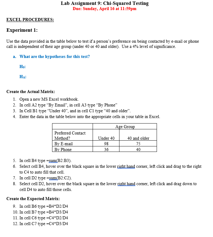
Lab Assignment 9: Chi-Squared Testing

Due: Sunday, April 16 at 11:59pm

EXCEL PROCEDURES:

Experiment 1:

Use the data provided in the table below to test if a person's preference on being contacted by e-mail or phone call is independent of their age group (under 40 or 40 and older). Use a 4% level of significance.

1. What are the hypotheses for this test?

H₀:

H_A:

Create the Actual Matrix:

1. Open a new MS Excel workbook.
2. In cell A2 type "By Email", in cell A3 type "By Phone"
3. In Cell B1 type "Under 40", and in cell C1 type "40 and older".
4. Enter the data in the table below into the appropriate cells in your table in Excel.

	Age Group
Preferred Contact Method?	Under 40	40 and older
By E-mail	98	75
By Phone	36	40

1. In cell B4 type =sum(B2:B3).
2. Select cell B4, hover over the black square in the lower right hand corner, left click and drag to the right to C4 to auto fill that cell.
3. In cell D2 type =sum(B2:C2).
4. Select cell D2, hover over the black square in the lower right hand corner, left click and drag down to cell D4 to auto fill those cells.

Create the Expected Matrix:

1. In cell B6 type =B4*D2/D4
2. In cell B7 type =B4*D3/D4
3. In cell C6 type =C4*D2/D4
4. In cell C7 type =C4*D3/D4

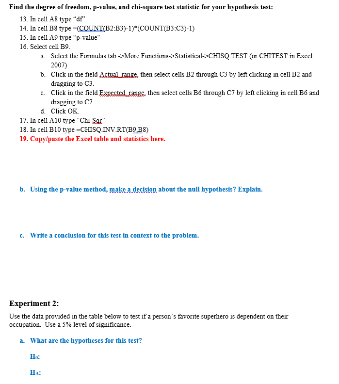
Find the degree of freedom, p-value, and chi-square test statistic for your hypothesis test:

1. In cell A8 type "df"
2. In cell B8 type =(COUNT(B2:B3)-1)*(COUNT(B3:C3)-1)
3. In cell A9 type "p-value"
4. Select cell B9.
   1. Select the Formulas tab ->More Functions->Statistical->CHISQ.TEST (or CHITEST in Excel 2007)
   2. Click in the field Actual_range, then select cells B2 through C3 by left clicking in cell B2 and dragging to C3.
   3. Click in the field Expected_range, then select cells B6 through C7 by left clicking in cell B6 and dragging to C7.
   4. Click OK.
5. In cell A10 type "Chi-Sqr"
6. In cell B10 type =CHISQ.INV.RT(B9,B8)
7. Copy/paste the Excel table and statistics here.

1. Using the p-value method, make a decision about the null hypothesis? Explain.

1. a conclusion for this test in context to the problem.

Experiment 2:

Use the data provided in the table below to test if a person's favorite superhero is dependent on their occupation. Use a 5% level of significance.

1. What are the hypotheses for this test?

H₀:

H_A:

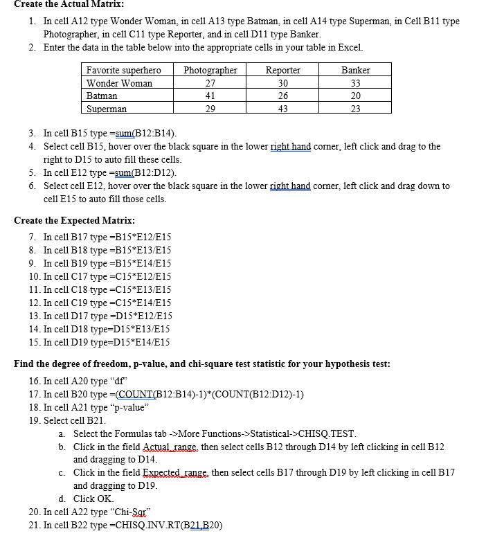
Create the Actual Matrix:

1. In cell A12 type Wonder Woman, in cell A13 type Batman, in cell A14 type Superman, in Cell B11 type Photographer, in cell C11 type Reporter, and in cell D11 type Banker.
2. Enter the data in the table below into the appropriate cells in your table in Excel.

Favorite superhero	Photographer	Reporter	Banker
Wonder Woman	27	30	33
Batman	41	26	20
Superman	29	43	23

1. In cell B15 type =sum(B12:B14).
2. Select cell B15, hover over the black square in the lower right hand corner, left click and drag to the right to D15 to auto fill these cells.
3. In cell E12 type =sum(B12:D12).
4. Select cell E12, hover over the black square in the lower right hand corner, left click and drag down to cell E15 to auto fill those cells.

Create the Expected Matrix:

1. In cell B17 type =B15*E12/E15
2. In cell B18 type =B15*E13/E15
3. In cell B19 type =B15*E14/E15
4. In cell C17 type =C15*E12/E15
5. In cell C18 type =C15*E13/E15
6. In cell C19 type =C15*E14/E15
7. In cell D17 type =D15*E12/E15
8. In cell D18 type=D15*E13/E15
9. In cell D19 type=D15*E14/E15

Find the degree of freedom, p-value, and chi-square test statistic for your hypothesis test:

1. In cell A20 type "df"
2. In cell B20 type =(COUNT(B12:B14)-1)*(COUNT(B12:D12)-1)
3. In cell A21 type "p-value"
4. Select cell B21.
   1. Select the Formulas tab ->More Functions->Statistical->CHISQ.TEST.
   2. Click in the field Actual_range, then select cells B12 through D14 by left clicking in cell B12 and dragging to D14.
   3. Click in the field Expected_range, then select cells B17 through D19 by left clicking in cell B17 and dragging to D19.
   4. Click OK.
5. In cell A22 type "Chi-Sqr"
6. In cell B22 type =CHISQ.INV.RT(B21,B20)
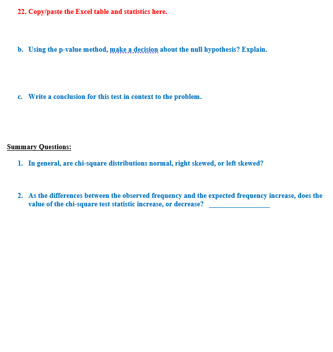
7. Copy/paste the Excel table and statistics here.

1. Using the p-value method, make a decision about the null hypothesis? Explain.

1. Write a conclusion for this test in context to the problem.

Summary Questions:

1. In general, are chi-square distributions normal, right skewed, or left skewed?

1. As the differences between the observed frequency and the expected frequency increase, does the value of the chi-square test statistic increase, or decrease? _________________

Lab Assignment 9: Chi-Squared Testing Due: Sunday, April 16 at 11:59pm EXCEL PROCEDURES: Experiment 1: Use the data provided in the table below to test if a person's preference on being contacted by e-mail or phone call is independent of their age group (under 40 or 40 and older). Use a 4% level of significance. a. What are the hypotheses for this test? Ho: HA Create the Actual Matrix: 1. Open a new MS Excel workbook. 2. In cell A2 type "By Email", in cell A3 type "By Phone" 3. In Cell Bl type "Under 40", and in cell Cl type "40 and older". 4. Enter the data in the table below into the appropriate cells in your table in Excel. Age Group Preferred Contact Method? Under 40 40 and older By E-mail 98 75 By Phone 36 40 5. In cell B4 type =sum(B2:B3). 6. Select cell B4, hover over the black square in the lower right hand corner, left click and drag to the right to C4 to auto fill that cell 7. In cell D2 type =sum(B2:C2). 8. Select cell D2, hover over the black square in the lower right hand corner, left click and drag down to cell D4 to auto fill those cells. Create the Expected Matrix: 9. In cell Bo type =B4*D2/D4 10. In cell B7 type =B4*D3/D4 11. In cell Co type =C4*D2/D4 12. In cell C7 type =C4*D3/D4Find the degree of freedom, p-value, and chi-square test statistic for your hypothesis test: 13. In cell AS type "of 14. In cell B8 type =(COUNT(B2:B3)-1)*(COUNT(B3:C3)-1) 15. In cell A9 type "p-value" 16. Select cell B9. a. Select the Formulas tab ->More Functions->Statistical->CHISQ.TEST (or CHITEST in Excel 2007) b. Click in the field Actual range, then select cells B2 through C3 by left clicking in cell B2 and dragging to C3. c. Click in the field Expected range, then select cells B6 through C7 by left clicking in cell Bo and dragging to C7. d. Click OK 17. In cell A10 type "Chi-Sar" 18. In cell B10 type =CHISQ.INV.RT(B2,B8) 19. Copy/paste the Excel table and statistics here. b. Using the p-value method, make a decision about the null hypothesis? Explain. c. Write a conclusion for this test in context to the problem. Experiment 2: Use the data provided in the table below to test if a person's favorite superhero is dependent on their occupation. Use a 5% level of significance. a. What are the hypotheses for this test? Ho: HA:Create the Actual Matrix: 1. In cell A12 type Wonder Woman, in cell A13 type Batman, in cell A14 type Superman, in Cell Bl1 type Photographer, in cell Cl1 type Reporter, and in cell D11 type Banker. 2. Enter the data in the table below into the appropriate cells in your table in Excel. Favorite superhero Photographer Reporter Banker Wonder Woman 27 30 33 Batman 41 26 20 Superman 29 43 23 3. In cell B15 type =sum(B12:B14) 4. Select cell B15, hover over the black square in the lower right hand corner, left click and drag to the right to D15 to auto fill these cells. 5. In cell E12 type =sum(B12:D12). 6. Select cell E12, hover over the black square in the lower right hand corner, left click and drag down to cell E15 to auto fill those cells. Create the Expected Matrix: 7. In cell B17 type =B15*E12/E15 8. In cell B18 type =B15*E13/E15 9. In cell B19 type =B15*E14/E15 10. In cell C17 type =C15*E12/E15 11. In cell C18 type =C15*E13/E15 12. In cell C19 type =C15*E14/E15 13. In cell D17 type =D15*E12/E15 14. In cell D18 type=D15*E13/E15 15. In cell D19 type=D15*E14/E15 Find the degree of freedom, p-value, and chi-square test statistic for your hypothesis test: 16. In cell A20 type "df" 17. In cell B20 type =(COUNT(B12:B14)-1)*(COUNT(B12:D12)-1) 18. In cell A21 type "p-value" 19. Select cell B21. a . Select the Formulas tab ->More Functions->Statistical->CHISQ.TEST. b. Click in the field Actual range, then select cells B12 through D14 by left clicking in cell B12 and dragging to D14. c. Click in the field Expected range, then select cells B17 through D19 by left clicking in cell B17 and dragging to D19. d. Click OK 20. In cell A22 type "Chi-Sar" 21. In cell B22 type =CHISQ.INV.RT(B21,B20)22. Copy/paste the Excel table and statistics here. b. Using the p-value method, make a decision about the null hypothesis? Explain. c. Write a conclusion for this test in context to the problem. Summary Questions: 1. In general, are chi-square distributions normal, right skewed, or left skewed? 2. As the differences between the observed frequency and the expected frequency increase, does the value of the chi-square test statistic increase, or decrease