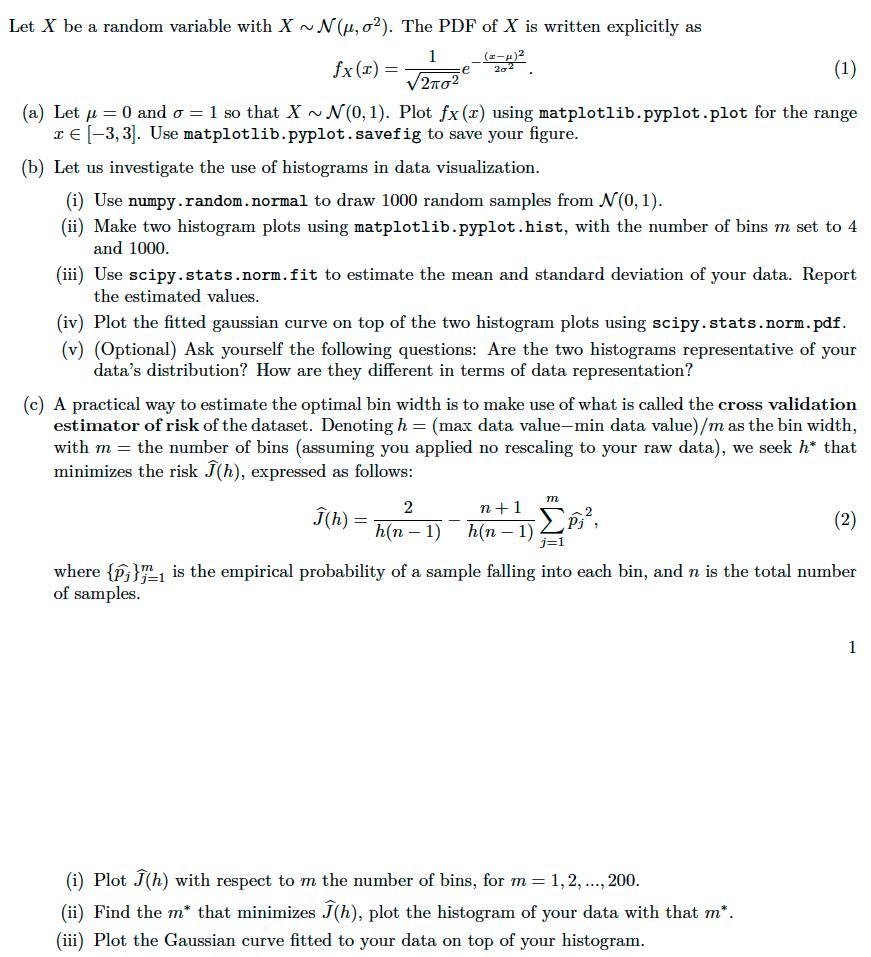
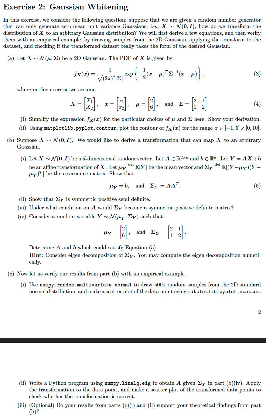
Let X be a random variable with X~ N(, 02). The PDF of X is written...
Fantastic news! We've Found the answer you've been seeking!
Question:
Transcribed Image Text:
Let X be a random variable with X~ N(μ, 02). The PDF of X is written explicitly as (2-μ)² fx(x) = (1) (a) Let μ = 0 and o= 1 so that X ~ N(0,1). Plot fx (r) using matplotlib.pyplot.plot for the range T€[-3,3]. Use matplotlib.pyplot.savefig to save your figure. (b) Let us investigate the use of histograms in data visualization. (i) Use numpy.random.normal to draw 1000 random samples from N(0, 1). (ii) Make two histogram plots using matplotlib.pyplot.hist, with the number of bins m set to 4 and 1000. 1 √2π0² e 202 (iii) Use scipy.stats.norm.fit to estimate the mean and standard deviation of your data. Report the estimated values. (iv) Plot the fitted gaussian curve on top of the two histogram plots using scipy.stats.norm.pdf. (v) (Optional) Ask yourself the following questions: Are the two histograms representative of your data's distribution? How are they different in terms of data representation? Ĵ(h) = (c) A practical way to estimate the optimal bin width is to make use of what is called the cross validation estimator of risk of the dataset. Denoting h= (max data value-min data value)/m as the bin width, with m = the number of bins (assuming you applied no rescaling to your raw data), we seek h* that minimizes the risk Ĵ(h), expressed as follows: m 2 n+1 h(n − 1) ¯ h(n − 1) ΣP₁², - j=1 (2) where {}1 is the empirical probability of a sample falling into each bin, and n is the total number of samples. (i) Plot Ĵ(h) with respect to m the number of bins, for m= = 1, 2, ..., 200. (ii) Find the m* that minimizes Ĵ(h), plot the histogram of your data with that m*. (iii) Plot the Gaussian curve fitted to your data on top of your histogram. 1 Exercise 2: Gaussian Whitening In this exercise, we consider the following question: suppose that we are given a random number generator that can only generate zero-mean unit variance Gaussians, i.e., X~ N(0, 1), how do we transform the distribution of X to an arbitrary Gaussian distribution? We will first derive a few equations, and then verify them with an empirical example, by drawing samples from the 2D Gaussian, applying the transform to the dataset, and checking if the transformed dataset really takes the form of the desired Gaussian. (a) Let X~ N(μ, E) be a 2D Gaussian. The PDF of X is given by 1 fx(x) = V(2π)2|Σ| where in this exercise we assume X₁ X₂ X = 7 x = [121] (i) Simplify the expression fx (x) for the particular choices of μ and Σ here. Show your derivation. (ii) Using matplotlib.pyplot.contour, plot the contour of fx (x) for the range x € [-1,5] x [0, 10]. transformation that can map X to an arbitrary exp {-} (x − µμ)²¹ ¶¯¹ (x − μµ)}}, (b) Suppose X~ N(0,1). We would like to derive Gaussian. μ = Hy = " and Σ= (3) (i) Let X ~ N(0, 1) be a d-dimensional random vector. Let A E Rdxd and be Rd. Let Y = AX +b be an affine transformation of X. Let py E[Y] be the mean vector and Ey Hy)] be the covariance matrix. Show that def def E[(Y-HY) (Y- Hy = b. and Xy = AAT. (ii) Show that Ey is symmetric positive semi-definite. (iii) Under what condition on A would Ey become a symmetric positive definite matrix? (iv) Consider a random variable Y~ N(y, Ey) such that (4) (5) and y = Determine A and b which could satisfy Equation (5). Hint: Consider eigen-decomposition of Ey. You may compute the eigen-decomposition numeri- cally. (c) Now let us verify our results from part (b) with an empirical example. (i) Use numpy.random.multivariate_normal to draw 5000 random samples from the 2D standard normal distribution, and make a scatter plot of the data point using matplotlib.pyplot.scatter. 2 (ii) Write a Python program using numpy.linalg.eig to obtain A given Ey in part (b)(iv). Apply the transformation to the data point, and make a scatter plot of the transformed data points to check whether the transformation is correct. (iii) (Optional) Do your results from parts (c) (i) and (ii) support your theoretical findings from part (b)? Let X be a random variable with X~ N(μ, 02). The PDF of X is written explicitly as (2-μ)² fx(x) = (1) (a) Let μ = 0 and o= 1 so that X ~ N(0,1). Plot fx (r) using matplotlib.pyplot.plot for the range T€[-3,3]. Use matplotlib.pyplot.savefig to save your figure. (b) Let us investigate the use of histograms in data visualization. (i) Use numpy.random.normal to draw 1000 random samples from N(0, 1). (ii) Make two histogram plots using matplotlib.pyplot.hist, with the number of bins m set to 4 and 1000. 1 √2π0² e 202 (iii) Use scipy.stats.norm.fit to estimate the mean and standard deviation of your data. Report the estimated values. (iv) Plot the fitted gaussian curve on top of the two histogram plots using scipy.stats.norm.pdf. (v) (Optional) Ask yourself the following questions: Are the two histograms representative of your data's distribution? How are they different in terms of data representation? Ĵ(h) = (c) A practical way to estimate the optimal bin width is to make use of what is called the cross validation estimator of risk of the dataset. Denoting h= (max data value-min data value)/m as the bin width, with m = the number of bins (assuming you applied no rescaling to your raw data), we seek h* that minimizes the risk Ĵ(h), expressed as follows: m 2 n+1 h(n − 1) ¯ h(n − 1) ΣP₁², - j=1 (2) where {}1 is the empirical probability of a sample falling into each bin, and n is the total number of samples. (i) Plot Ĵ(h) with respect to m the number of bins, for m= = 1, 2, ..., 200. (ii) Find the m* that minimizes Ĵ(h), plot the histogram of your data with that m*. (iii) Plot the Gaussian curve fitted to your data on top of your histogram. 1 Exercise 2: Gaussian Whitening In this exercise, we consider the following question: suppose that we are given a random number generator that can only generate zero-mean unit variance Gaussians, i.e., X~ N(0, 1), how do we transform the distribution of X to an arbitrary Gaussian distribution? We will first derive a few equations, and then verify them with an empirical example, by drawing samples from the 2D Gaussian, applying the transform to the dataset, and checking if the transformed dataset really takes the form of the desired Gaussian. (a) Let X~ N(μ, E) be a 2D Gaussian. The PDF of X is given by 1 fx(x) = V(2π)2|Σ| where in this exercise we assume X₁ X₂ X = 7 x = [121] (i) Simplify the expression fx (x) for the particular choices of μ and Σ here. Show your derivation. (ii) Using matplotlib.pyplot.contour, plot the contour of fx (x) for the range x € [-1,5] x [0, 10]. transformation that can map X to an arbitrary exp {-} (x − µμ)²¹ ¶¯¹ (x − μµ)}}, (b) Suppose X~ N(0,1). We would like to derive Gaussian. μ = Hy = " and Σ= (3) (i) Let X ~ N(0, 1) be a d-dimensional random vector. Let A E Rdxd and be Rd. Let Y = AX +b be an affine transformation of X. Let py E[Y] be the mean vector and Ey Hy)] be the covariance matrix. Show that def def E[(Y-HY) (Y- Hy = b. and Xy = AAT. (ii) Show that Ey is symmetric positive semi-definite. (iii) Under what condition on A would Ey become a symmetric positive definite matrix? (iv) Consider a random variable Y~ N(y, Ey) such that (4) (5) and y = Determine A and b which could satisfy Equation (5). Hint: Consider eigen-decomposition of Ey. You may compute the eigen-decomposition numeri- cally. (c) Now let us verify our results from part (b) with an empirical example. (i) Use numpy.random.multivariate_normal to draw 5000 random samples from the 2D standard normal distribution, and make a scatter plot of the data point using matplotlib.pyplot.scatter. 2 (ii) Write a Python program using numpy.linalg.eig to obtain A given Ey in part (b)(iv). Apply the transformation to the data point, and make a scatter plot of the transformed data points to check whether the transformation is correct. (iii) (Optional) Do your results from parts (c) (i) and (ii) support your theoretical findings from part (b)?
Expert Answer:
Answer rating: 100% (QA)
Exercise 1 a Plotting PDF of N0 1 Python import numpy as np import matplotlibpyplot as plt from scipystats import norm Parameters mu 0 sigma 1 x nplinspace3 3 1000 pdf normpdfx mu sigma Plotting pltpl... View the full answer
Related Book For
Posted Date:
Students also viewed these programming questions
-
Beginning inventory, purchases, and sales for Item Zeta9 are as follows: Oct. 1 Inventory 45 units @$24 7 Sale. 32 units 15 Purchase 31 units @ $28 24 Sale 19 units Assuming a perpetual inventory...
-
Let X be a random variable with pdf pX (k) = 1/n, for k = 0, 1, 2, . . . , n 1 and 0 otherwise. Show that MX(t) = 1ent/n(1 et).
-
Let X be a random variable with a Student's t distribution with p degrees of freedom. (a) Derive the mean and variance of X. (b) Show that X2 has an F distribution with 1 and p degrees of freedom....
-
A 14-foot piece of string is cut into two pieces so that the longer piece is 2 feet longer than twice the shorter piece. Find the lengths of both pieces. What is the lenath of the shorter oiece?1...
-
Focal Length of a Zoom Lens Figure 34.63 shows a simple version of a zoom lens. The converging lens has focal length f1, and the diverging lens has focal length f2 = ?? | f2|. The two lenses are...
-
Three brands of batteries are under study. It is suspected that the lives (in weeks) of the three brands are different. Five batteries of each brand are tested with the following results: (a) Are the...
-
After receiving complaints from readers, your campus newspaper decides to redesign its front page. A new format B is developed and tested against the current format, A. A total of 100 students are...
-
Charles River Associates is considering whether to call either of the two perpetual bond issues the company currently has outstanding. If the bond is called, it will be refunded, that is, a new bond...
-
Prepare adjusting entries for the following transactions (use the worksheet on next page), assuming all normal journal entries during the year has already been made. You are now at yea end (i.e.,...
-
On December 31, the Income Summary account of Johnson Company has a Credit balance of $226,000 after revenue of $519,000 and expenses of $293,000 were closed to the account. Gloria Johnson, Drawing...
-
Determine the displacement midway between the supports for the overhang- ing beam. a- FIG. P6.32
-
WHY IS CREDIT CALLED AS A PRODUCTIVE ASSET THAT MUST BE MANAGED WITH A BANK'S PROPERTIES?
-
In your initial post of including references in APA , describe three ways in which data are used in business functions. Use one way data is used in Accounting, one way in Marketing and one way in...
-
DANELLA DANCE studios is evaluating the purchase of new sound equipment that will increase the probability of your aerobic dances. The equipment will cost $28,000. Danells is not sure how many...
-
Why does the coupon bond price suddenly drop after a coupon payment?
-
Answer these questions on business ethics "What do people stand for?" "What is ethical business?" "How do values support personal code of ethics?" Provide a statement of ethics as it pertains to...
-
The value of F-dr, where F = (x+z)i +(2y-z)j + (x-2)k and Cis the boundary of the triangle with vertices P(6.0.0), Q(0, 4, 0) and R(0, 0, 3) is 6 24 36 0
-
C- Consider the following scenario:- A supermarket needs to develop the following software to encourage regular customers. For this, the customer needs to supply his/her residence address, telephone...
-
Let X be a single observation from the beta(, 1) pdf. a. Let Y = - (logX)-1. Evaluate the confidence coefficient of the set [y/2, y]. b. Find a pivotal quantity and use it to set up a confidence...
-
(a) Suppose it is desired to generate Y ~ beta(o, b), where a and b are not integers. Show that using V ~ beta([a], |b]) will result in a finite value of M = suPy, fy (y)j fv (y). (b) Suppose it is...
-
(a) For the hierarchy in Example 4.4.6, show that the marginal distribution of X is given by the beta-binomial distribution, (b) A variation on the hierarchical model in part (a) is X|P ~ negative...
-
Demonstrate that for colors \(r, g\), and \(b\), color \(\mathrm{SU}(3)\) two-quark states are of the form \(q q=\mathbf{3} \otimes \mathbf{3}=\mathbf{6} \oplus \overline{\mathbf{3}}\), with Show...
-
Verify the color SU(3) representations for combinations of three or fewer quarks and antiquarks given in Eq. (19.28). Data from Eq. 19.28 qq=303=108 qq 3 3 603, 999 3 3 3 = 36315, qqq 3 3 3 1088 10,
-
Prove that Eq. (19.34) gives the simplest multi-gluon and gluon-quark states that contain an \(\mathrm{SU}(3)\) color singlet in the decomposition. Data from Eq. 19.34 (GG)1: (88)1 (Gqq) : [8 (383)8]...
Study smarter with the SolutionInn App