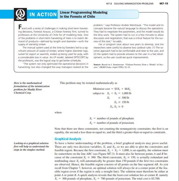
M7.8 SOLVING MINIMIZATION PROBLEMSM 7-19 IN ACTION Linear Programming Modeling in the Forests of Chile aced with a series of challenges in making short-term harvest ing decisions, Forestal Arauco, a Chilean forestry firm, turned to professors at the University of Chile for LP modeling help. One of the problems in short-term harvesting of trees is to match de- mand of products-defined by length and diameter-with the Supply of standing timber The manual system used at the time by foresters led to a sig- nificant amount of waste of timber, where higher diameter logs. suited for export or sawmills, ended up being used for pulp, with a considerable loss in value. An LP model, labeled OPTICORT by the professors, was the logical way to get better schedules The system not only optimazed the operational decisions in harvesting, but also changed the way managers looked at the problem," says Professor Andres Weintraub "The model and its concepts became the natural language to discuss the operations They had to negotiate the parameters, and the model would do the dirty work. The systern had to run in a few minutes to allow discussion and negotiation, that was a critical feature for the suc- cess of this tool," he adds. The LP program took about two years to develop, and the researchers were careful to observe two cardinal rules (1) The so- lution approach had to be comfortable and clear to the user, and 21 the system had to provide answers to the user in a fast devel- Opment, so the user could see quick improvements. 'Model of Suc- Source: Based on . Sumnerour Chilean Forestry Farm cess," OR MS Today April 1999 22-23 This problem may be restated mathematically as Here is the mathematical formulation of the minimization problem for Muddy River Chemical Corp Minimize cost = $5X, + $6X subject to X1 + X = 1,000 lb x 30016 X 150 lb X, X, 20 where Xi = number of pounds of phosphate X = number of pounds of potassium Note that there are three constraints, not counting the nonnegativity constraints, the first is an equality, the second a less-than-or-equal-to, and the third a greater than-or-equal to constraint. Looking at a graphical solution first will help us understand the steps in the simplex method. Graphical Analysis To have a better understanding of the problem. a brief graphical analysis may prove useful. There are only two decision variables, X and X, so we are able to plot the constraints and feasible region. Because the first constraint. X + x = 1.0XX), is an equality, the solution must lie somewhere on the line ABC (see Figure M7.3). It must also lie between points A and B be- cause of the constraint X 300. The third constraint. X 150, is actually redundant and nonbinding since X, will automatically be greater than 150 pounds if the first two constraints are observed. Hence, the feasible region consists of all points on the line segment AB. As you recall from Chapter 7, however, an optimal solution will always lie at a comer point of the fea- sible region (even if the region is only a straight line). The solution must therefore be either at point A or point B. A quick analysis reveals that the least-cost solution lies at corner B, namely X = 300 pounds of phosphate. X, = 700 pounds of potassium. The total cost is $5.700