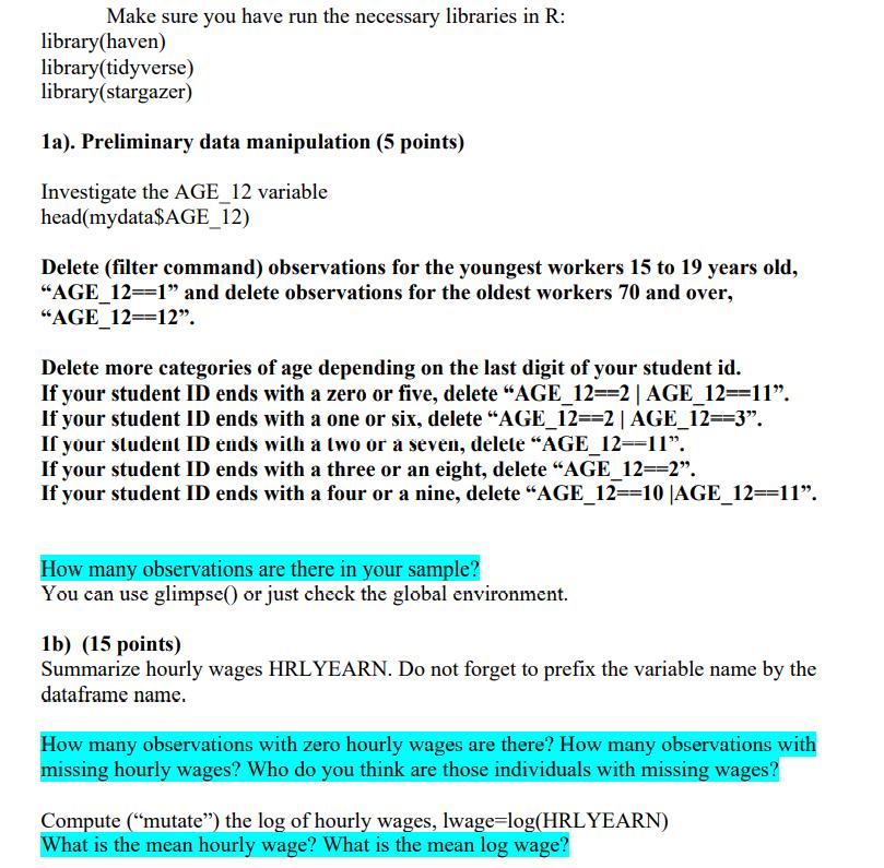
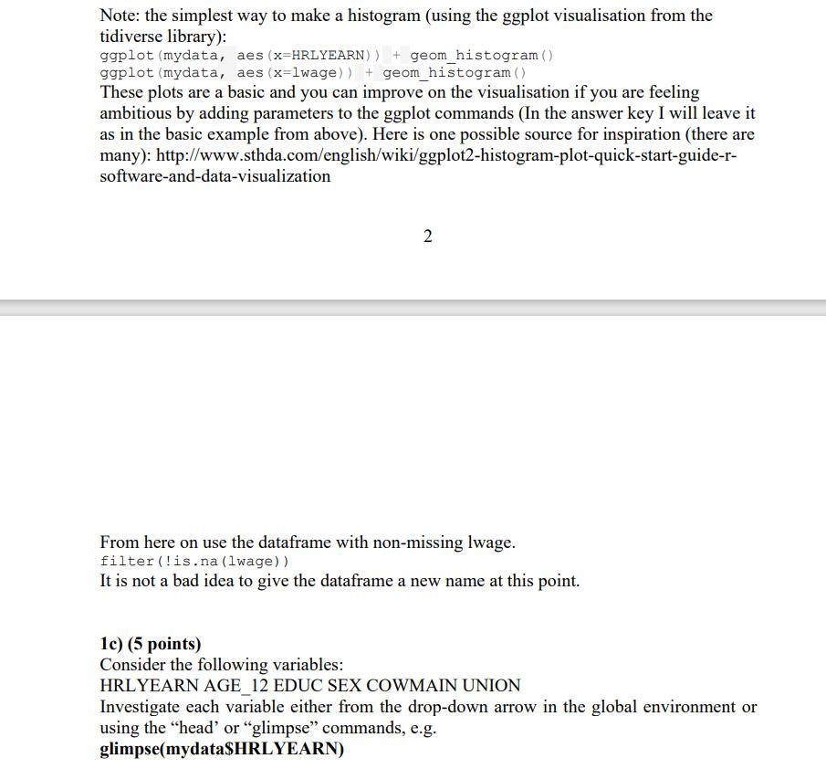
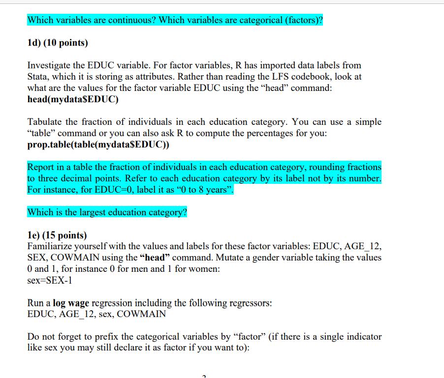
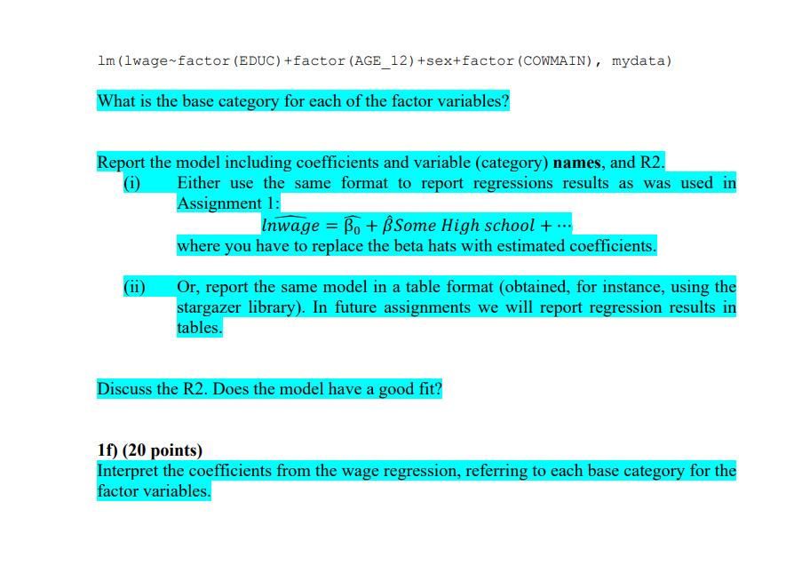
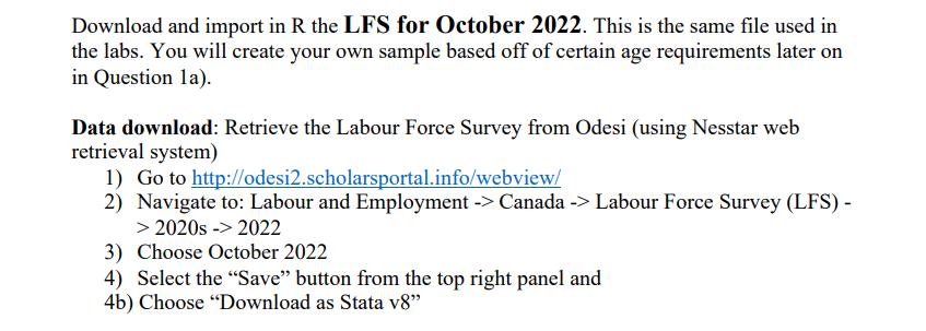
Make sure you have run the necessary libraries in R: library(haven) library(tidyverse) library(stargazer) 1a). Preliminary data manipulation (5 points) Investigate the AGE_12 variable head(mydata$AGE_12) Delete (filter command) observations for the youngest workers 15 to 19 years old, "AGE_12=1" and delete observations for the oldest workers 70 and over, "AGE_12=12". Delete more categories of age depending on the last digit of your student id. If your student ID ends with a zero or five, delete "AGE_12=-2 |AGE_12==11". If your student ID ends with a one or six, delete "AGE_12==2 | AGE_12==3. If your student ID ends with a two or a seven, delete "AGE_12--11". If your student ID ends with a three or an eight, delete "AGE_12==2". If your student ID ends with a four or a nine, delete "AGE_12=-10 |AGE_12=11". How many observations are there in your sample? You can use glimpse() or just check the global environment. 1b) (15 points) Summarize hourly wages HRLYEARN. Do not forget to prefix the variable name by the dataframe name. How many observations with zero hourly wages are there? How many observations with missing hourly wages? Who do you think are those individuals with missing wages? Compute ("mutate") the log of hourly wages, lwage=log(HRLYEARN) What is the mean hourly wage? What is the mean log wage? Note: the simplest way to make a histogram (using the ggplot visualisation from the tidiverse library): ggplot (mydata, aes (x-HRLYEARN)) + geom_histogram () ggplot (mydata, aes (x=lwage)) + geom_histogram () These plots are a basic and you can improve on the visualisation if you are feeling ambitious by adding parameters to the ggplot commands (In the answer key I will leave it as in the basic example from above). Here is one possible source for inspiration (there are many): http://www.sthda.com/english/wiki/ggplot2-histogram-plot-quick-start-guide-r- software-and-data-visualization 2 From here on use the dataframe with non-missing lwage. filter (!is.na (lwage)) It is not a bad idea to give the dataframe a new name at this point. 1c) (5 points) Consider the following variables: HRLYEARN AGE_12 EDUC SEX COWMAIN UNION Investigate each variable either from the drop-down arrow in the global environment or using the "head" or "glimpse" commands, e.g. glimpse(mydata$HRLYEARN) Which variables are continuous? Which variables are categorical (factors)? 1d) (10 points) Investigate the EDUC variable. For factor variables, R has imported data labels from Stata, which it is storing as attributes. Rather than reading the LFS codebook, look at what are the values for the factor variable EDUC using the "head" command: head(mydata$EDUC) Tabulate the fraction of individuals in each education category. You can use a simple "table" command or you can also ask R to compute the percentages for you: prop.table(table(mydata$EDUC)) Report in a table the fraction of individuals in each education category, rounding fractions to three decimal points. Refer to each education category by its label not by its number. For instance, for EDUC=0, label it as "0 to 8 years". Which is the largest education category? 1e) (15 points) Familiarize yourself with the values and labels for these factor variables: EDUC, AGE_12, SEX, COWMAIN using the "head" command. Mutate a gender variable taking the values O and 1, for instance 0 for men and 1 for women: sex-SEX-1 Run a log wage regression including the following regressors: EDUC, AGE_12, sex, COWMAIN Do not forget to prefix the categorical variables by "factor" (if there is a single indicator like sex you may still declare it as factor if you want to): 1m (1wage factor (EDUC) +factor (AGE_12) +sex+factor (COWMAIN), mydata) What is the base category for each of the factor variables? Report the model including coefficients and variable (category) names, and R2. Either use the same format to report regressions results as was used in Assignment 1: (i) (ii) Inwage=Bo+ Some High school+... where you have to replace the beta hats with estimated coefficients. Or, report the same model in a table format (obtained, for instance, using the stargazer library). In future assignments we will report regression results in tables. Discuss the R2. Does the model have a good fit? 1f) (20 points) Interpret the coefficients from the wage regression, referring to each base category for the factor variables. Download and import in R the LFS for October 2022. This is the same file used in the labs. You will create your own sample based off of certain age requirements later on in Question la). Data download: Retrieve the Labour Force Survey from Odesi (using Nesstar web retrieval system) 1) Go to http://odesi2.scholarsportal.info/webview/ 2) Navigate to: Labour and Employment -> Canada -> Labour Force Survey (LFS) - > 2020s -> 2022 3) Choose October 2022 4) Select the "Save" button from the top right panel and 4b) Choose "Download as Stata v8"