(MATLAB)

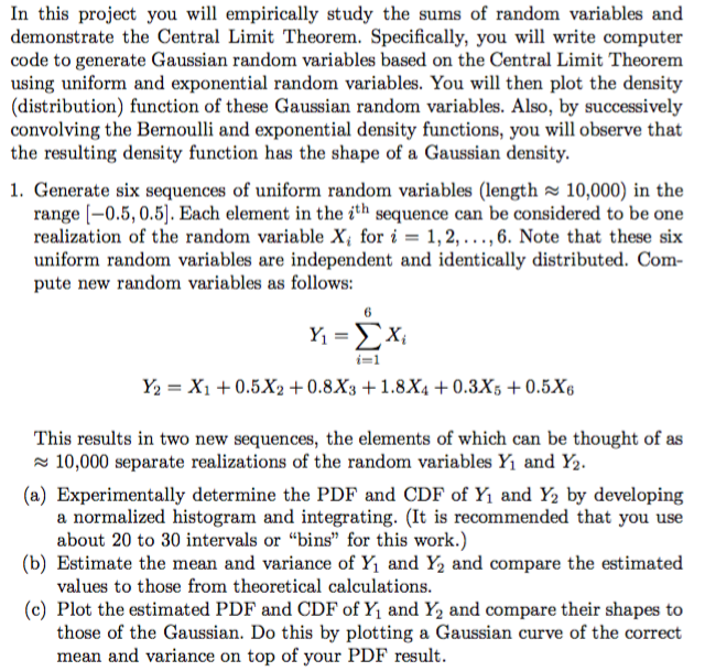
In this project you will empirically study the sums of random variables and demonstrate the Central Limit Theorem. Specifically, you will write computer code to generate Gaussian random variables based on the Central Limit Theorem using uniform and exponential random variables. You will then plot the density (distribution) function of these Gaussian random variables. Also, by successively convolving the Bernoulli and exponential density functions, you will observe that the resulting density function has the shape of a Gaussian density. Generate six sequences of uniform random variables (length 10,000) in the range [-0.5,0.5]. Bach element in the i^th sequence can be considered to be one realization of the random variable A, for i = 1,2, ...,6. Note that these six uniform random variables are independent and identically distributed. Compute new random variables as follows: Y_1 sigma_i=1^6 X_i Y_2 = X_1 + 0.5 X_2 + 0.8 X_3 + 1.8 X_4 + 0.3 X_5 + 0.5 X_6 This results in two new sequences, the elements of which can be thought of as 10,000 separate realizations of the random variables Y_1 and Y_2. Experimentally determine the PDF and CDF of Y_1 and Y_2 by developing a normalized histogram and integrating. (It is recommended that you use about 20 to 30 intervals or "bins" for this work.) Estimate the mean and variance of Y_1 and Y_2 and compare the estimated values to those from theoretical calculations. Plot the estimated PDF and CDF of Y_1 and Y_2 and compare their shapes to those of the Gaussian. Do this by plotting a Gaussian curve of the correct mean and variance on top of your PDF result. In this project you will empirically study the sums of random variables and demonstrate the Central Limit Theorem. Specifically, you will write computer code to generate Gaussian random variables based on the Central Limit Theorem using uniform and exponential random variables. You will then plot the density (distribution) function of these Gaussian random variables. Also, by successively convolving the Bernoulli and exponential density functions, you will observe that the resulting density function has the shape of a Gaussian density. Generate six sequences of uniform random variables (length 10,000) in the range [-0.5,0.5]. Bach element in the i^th sequence can be considered to be one realization of the random variable A, for i = 1,2, ...,6. Note that these six uniform random variables are independent and identically distributed. Compute new random variables as follows: Y_1 sigma_i=1^6 X_i Y_2 = X_1 + 0.5 X_2 + 0.8 X_3 + 1.8 X_4 + 0.3 X_5 + 0.5 X_6 This results in two new sequences, the elements of which can be thought of as 10,000 separate realizations of the random variables Y_1 and Y_2. Experimentally determine the PDF and CDF of Y_1 and Y_2 by developing a normalized histogram and integrating. (It is recommended that you use about 20 to 30 intervals or "bins" for this work.) Estimate the mean and variance of Y_1 and Y_2 and compare the estimated values to those from theoretical calculations. Plot the estimated PDF and CDF of Y_1 and Y_2 and compare their shapes to those of the Gaussian. Do this by plotting a Gaussian curve of the correct mean and variance on top of your PDF result