

Question: Melbourne Client List Each question below has one correct answer. Select the correct answer by changing the FALSE to TRUE. 3 The Last Order Dates
Melbourne Client List
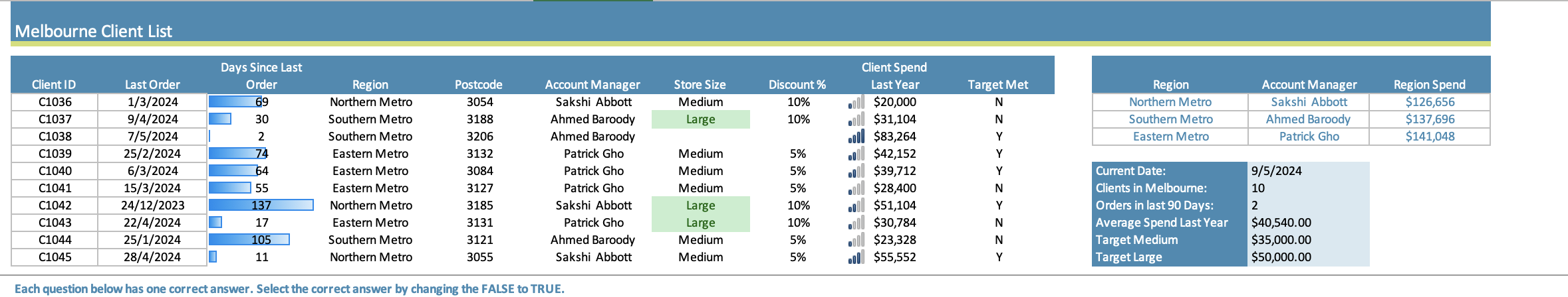
Each question below has one correct answer. Select the correct answer by changing the FALSE to TRUE. The Last Order Dates have been changed to centre align, by default they would align:
A Top Left
FALSE
B Top Right
FALSE
C Bottom Left
FALSE
D Bottom Right
the Formula AVERAGEJ will equal:
A
FALSE
B
FALSE
C #DIV
FALSE
D
FALSE
Which syntax is NOT correct for adding values in cells and
A
FALSE
B :
FALSE
D :
FALSE
FALSE
returns which answer?
A
FALSE
B
FALSE
C
FALSE
D
FALSE
Which of the following would calculate the most recent Order Date?
A RECENTC:C
B DATEC:C
C VLOOKUPC:C
D MAx: The cells H: are empty. What will the formaula COUNTH: return?
A
B An error
C
D
Which of the following statements about named ranges is true?
A Named ranges automatically extend to include values added directly to the right.
FALSE
B Named ranges automatically extend to include values added directly below.
C If you change the name or range of a named range, all formulas using it will update.
D If you delete a named range, formulas will revert to using original cell references.
Which of the following options is NOT available on the Tables ribbon?
A Insert Slicer
B Remove Duplicates
C Add Column
D Convert to Range
When you first opened this workbook, which was true?
A There are no tables
B There are no named ranges or tables
C There are no named ranges
D There are more tables than named ranges
Which chart type would be the best to show daily stock prices over a year?
A Pie Chart
B Line Chart
C Stacked Bar Chart Which Highlight cell values Conditional formatting rule could have been applied to H:H
A Greater Than
FALSE
B Less Than
C Duplicates
D Equal To
Which calculation will return the number of customers who have NOT placed an order in the last days?
A COUNTIFD:D
FALSE
B COUNTIFSD:D
C COUNTIFSD:D
D COUNTIFD:D
The following formula AVERAGEIFSD:DF:F will return...
A
B
C
D An Error
FALSE
What will the formula return?
A
B
C
D FALSE
FALSE
The correct formula to calculate if Medium and Large stores achieved their targets is
A IFH"Large",IFJYNIFJYN
B IFANDH"Large",JYANDH"Medium",JYN
C IFORH"Large",JYORH"Medium",JYN
D IFSH"Large","YJYNH"Medium","YJYN Which formula would calculate the total spend for just the Northern and Southern Metro Areas?
A SUMIFE:EJ:J"Northern Metro" & "Southern Metro"
B SUMIFSJ:JE:EORNorthern Metro","Southern Metro"
SUMIFSJ:JE:EEastern Metro"
FALSE
D SUMIFJ:JE:E"Northern Metro" AND "Southern Metro"
FALSE
FALSE
FALSE
Using the formula VLOOKUP : to return the last year spend for client at postcode is incorrect...
A because should be in quotation marks, ie
FALSE
B because the look up range should be B:K
FALSE
C because it should be an exact match
FALSE
D because it should use absolute cell referencing
FALSE
The formula VLOOKUPCB:JIFD will return
A
B
C
D
FALSE
FALSE
FALSE
FALSE
Step by Step Solution
There are 3 Steps involved in it
1 Expert Approved Answer
Step: 1 Unlock

Question Has Been Solved by an Expert!
Get step-by-step solutions from verified subject matter experts
Step: 2 Unlock
Step: 3 Unlock