My professor includes a "test script" for us to write our code in and test it, I have included it below

'''implement three ways to evaluate a degree m polynomial pm(x) = c[0] + c[1]*x + ... c[m]*x**m . at x, and reurn the polynomial value pm(x). the m should be determined from the length of the input vector c.

note 1: for each input c, the polynomial is assumed to be c[0] + c[1]*x + ... c[m]*x**m, not the other form c[0]*x**m + c[1]*x**(m-1) + ... + c[m] which is also often used. note 2: if x is a vector, then the returned value should be a vector of same length as x. '''

import numpy as np

def polym(c, x): # this function evaluates c[0] + c[1]*x + ... c[m]*x**m by summing term by term, # it computes x**i at the i-th iteration (the slowest of all of the three methods) # #make sure x is an np array so that it can be scaled (i.e., x*x will be x**2 elementwisely)

def polym2(c, x): # this function evaluates c[0] + c[1]*x + ... c[m]*x**m by summing term by term, # it should not compute x**i directly at each iteration, instead it should update # x**i as x**(i-1)*x, reusing the x**(i-1) that is already computed at the previous iteration # #make sure x is an np array so that it can be scaled (i.e., x*x will be x**2 elementwisely) #(also, be careful when copying an np array, if not done properly, it would be hard to debug)

def horner(c, x): # this function evaluates c[0] + c[1]*x + ... c[m]*x**m by the Horner's method. #make sure x is an np array so that it can be scaled (i.e., x*x will be x**2 elementwisely)

def compare_efficiency():

import time print(' ==> Now compare the efficiency of the methods: ') mmin=4000; mmax=20000; step=2000

#initialize lists to store the time for each method time_poly=[]; time_poly2=[]; time_horner=[] for m in range(mmin, mmax, step): c = np.random.randn(m) x = np.random.randn(round(m/4)); x /= max(abs(x))

#using the above generated x and c, #add code below to call the three functions above, find the excution time for each, #and store the time in the corresponding lists

#add code to print out the timing info using the format specified in the project PDF file

x= range(mmin, mmax, step) #add code below to plot the figure using the format specified in the project PDF file

#add code save the plot into a file naed 'poly_eval_compare.png' for submission

#========================================================================== #do not modify code below this line def accuracy_check(c, x, tol=1e-8): failcount=0 p1 = polym(c, x) p2 = polym2(c, x) p3 = horner(c, x) print(' by polym: {}, by polym2:{}, by horner:{}'.format(p1, p2, p3)) if max(abs((p1 - p3)/p3)) > tol: print(' **** error in either polym() or horner() *** '); failcount+=1 elif max(abs((p2 - p3)/p3)) > tol: print(' **** error in either polym2() or horner() *** '); failcount+=1 elif max(abs((p1 - p2)/p1)) > tol: print(' **** error in polym() or polym2() *** '); failcount+=1 else: print(' Well done, polynomial values by all methods are the same ! ')

return failcount

if __name__=='__main__':

import matplotlib.pyplot as plt fcount = 0 pf = lambda x: np.pi + x**6 - x**9 + np.e*x**10 c = [np.pi, 0, 0, 1, 0, -1, 0, 0, 0, 0, np.e]; x= [-0.8, 0.9] print(' Test 1:'); fcount += accuracy_check(c, x) c = np.random.randint(-100, 100, size=(61))/1.; x = np.random.rand(10) print(' Test 2:'); fcount += accuracy_check(c, x)

k = 3 for m in range(2, 350, 20): c = np.random.randn(m); x = np.random.randn(12) print(' Test {} on degree {} polynomial'.format(k, m)) fcount += accuracy_check(c, x) k+=1

if fcount == 0: print(' Congratulations for passing all tests. ') else: print(" Total number of failed tests={}, need more debugging".format(fcount))

#compare the time efficiency (evaluting higher degree polynomials at many points) #(you may want to comment out the flowing line whe debuging to pass the above tests) compare_efficiency()

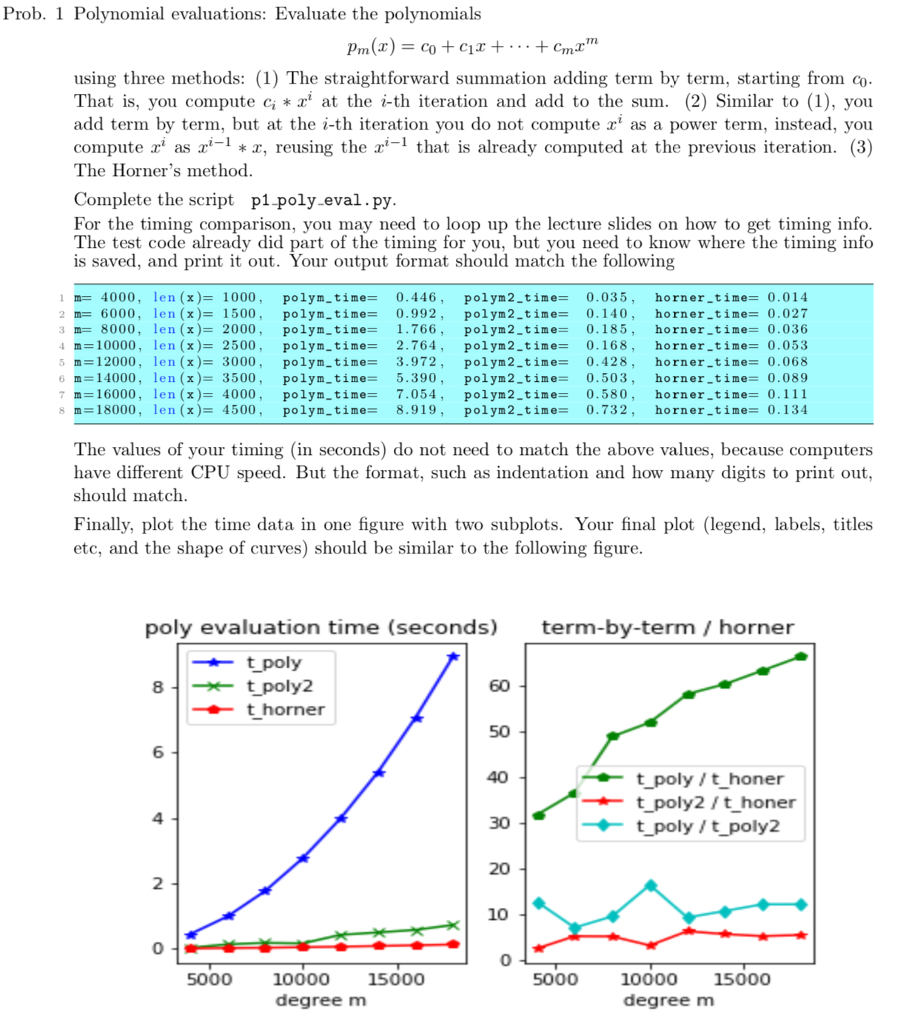
Prob. 1 Polynomial evaluations: Evaluate the polvnomials using three methods: (1) The straightforward summation adding term by term, starting from co That is, you compute at the i-th iteration and add to the sum. (2) Similar to (1), you add term by term, but at the i-th iteration you do not compute r1 as a power term, instead, you compute a as z, reusing the -1 that is already computed at the previous iteration. (3) The Horner's method Complete the script p1-poly eval.py For the timing comparison, you may need to loop up the lecture slides on how to get timing info The test code already did part of the timing for you, but you need to know where the timing info is saved, and print it out. Your output format should match the following 1 m=4000, 2 m=6000, 3m=8000, im=10000, 5m=12000, 6m-14000 , 7m=16000, sm=18000, len (x)= 1000, len(x)= 1500, len (x)= 2000, len (x)=2500, len (x)-3000, len (x)=3500, len (x)= 4000, len (x)-4500, polym-time= polym-time= polym-time= polym-time= polym-time= polym-time= polym-time= polym-time= 0.446, 0.992, 1.766, 2.764 , 3.972, 5.390, 7.054 , 8.919, polym2-time= polym2-time= polym2-time= polym2-time= polym2-time= polyn2-time= polym2-time= polym 2-time= 0.035, 0.140, 0.185, 0.168, 0.428, 0.503, 0.580, 0.732, horner-time= horner-time= horner-time= horner-time= horner-time= horner-time= horner-time= horner-time= 0.014 0.027 0.036 0.053 0.068 0.089 0.111 0.134 The values of your timing (in seconds) do not need to match the above values, because computers have different CPU speed. But the format, such as indentation and how many digits to print out, should match Finally, plot the time data in one figure with two subplots. Your final plot (legend, labels, titles etc, and the shape of curves) should be similar to the following figure. poly evaluation time (seconds) term-by-term /horner 60 t horner 50 6 40 t poly/t honer t poly2/t_honer t poly/t poly2 4 30 20 2 10 0 0 5000 10000 15000 degree m 5000 10000 15000 degree m