need assistance with this spreadsheet

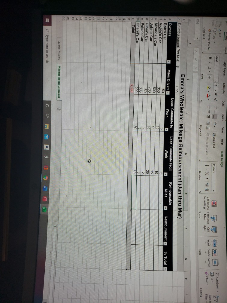
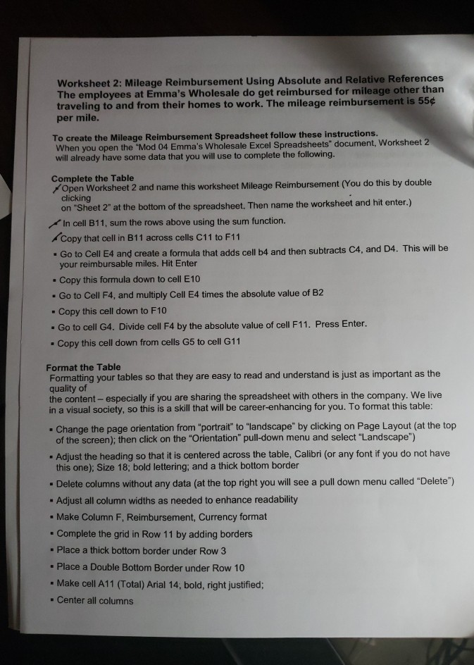
Home Insert Page Layout Formulas Data Review View Help Table Design Arial 12 - A A EEP- 95 Wrap Text Xcul In Copy - 3 Format Painter Clipboard Custom IE BIU A Merge & Center $ 5 Autosum - Am ZY Sort 8 Clear Filter- Editing %. Insert Delete Format Conditional Format as Cell Formatting Table Styles Styles Font Alignment Number Cells E10 G H 1 Reimbursement Per Mile: % Total Owners Bob's Car 5 Vickie's Car 6 Miranda's Car 7 John's Car 8 Olivia's Car Peter's Car Cheryl's Car 11 Total 12 13 D Emma's Wholesale: Mileage Reimbursement (Jan thru Mar) s 0.55 Less: Commute to Less: Commute From Reimbursable Miles Driven Work Work - Miles Reimbursment 150 5 5 350 10 10 500 15 15 700 20 20 50 2 2 600 3 3 1.000 50 50 3.350 15 16 17 18 19 20 21 22 23 24 25 26 27 Quarterly Sales Mileage Reimbursement Type here to search O a w Worksheet 2: Mileage Reimbursement Using Absolute and Relative References The employees at Emma's Wholesale do get reimbursed for mileage other than traveling to and from their homes to work. The mileage reimbursement is 55 per mile. To create the Mileage Reimbursement Spreadsheet follow these instructions. When you open the "Mod 04 Emma's Wholesale Excel Spreadsheets" document, Worksheet 2 will already have some data that you will use to complete the following. Complete the Table Open Worksheet 2 and name this worksheet Mileage Reimbursement (You do this by double clicking on "Sheet 2" at the bottom of the spreadsheet. Then name the worksheet and hit enter.) In cell B11, sum the rows above using the sum function. Copy that cell in B11 across cells C11 to F11 . Go to Cell E4 and create a formula that adds cell b4 and then subtracts C4, and D4. This will be your reimbursable miles. Hit Enter Copy this formula down to cell E10 . Go to Cell F4, and multiply Cell E4 times the absolute value of B2 Copy this cell down to F10 . Go to cell G4. Divide cell F4 by the absolute value of cell F11. Press Enter. Copy this cell down from cells G5 to cell G11 . . . Format the Table Formatting your tables so that they are easy to read and understand is just as important as the quality of the content - especially if you are sharing the spreadsheet with others in the company. We live in a visual society, so this is a skill that will be career-enhancing for you. To format this table: Change the page orientation from "portrait" to "landscape" by clicking on Page Layout (at the top of the screen); then click on the "Orientation" pull-down menu and select "Landscape") - Adjust the heading so that it is centered across the table, Calibri (or any font if you do not have this one); Size 18; bold lettering, and a thick bottom border Delete columns without any data (at the top right you will see a pull down menu called "Delete") - Adjust all column widths as needed to enhance readability - Make Column F, Reimbursement, Currency format Complete the grid in Row 11 by adding borders - Place a thick bottom border under Row 3 - Place a Double Bottom Border under Row 10 - Make cell A11 (Total) Arial 14, bold, right justified; - Center all columns Home Insert Page Layout Formulas Data Review View Help Table Design Arial 12 - A A EEP- 95 Wrap Text Xcul In Copy - 3 Format Painter Clipboard Custom IE BIU A Merge & Center $ 5 Autosum - Am ZY Sort 8 Clear Filter- Editing %. Insert Delete Format Conditional Format as Cell Formatting Table Styles Styles Font Alignment Number Cells E10 G H 1 Reimbursement Per Mile: % Total Owners Bob's Car 5 Vickie's Car 6 Miranda's Car 7 John's Car 8 Olivia's Car Peter's Car Cheryl's Car 11 Total 12 13 D Emma's Wholesale: Mileage Reimbursement (Jan thru Mar) s 0.55 Less: Commute to Less: Commute From Reimbursable Miles Driven Work Work - Miles Reimbursment 150 5 5 350 10 10 500 15 15 700 20 20 50 2 2 600 3 3 1.000 50 50 3.350 15 16 17 18 19 20 21 22 23 24 25 26 27 Quarterly Sales Mileage Reimbursement Type here to search O a w Worksheet 2: Mileage Reimbursement Using Absolute and Relative References The employees at Emma's Wholesale do get reimbursed for mileage other than traveling to and from their homes to work. The mileage reimbursement is 55 per mile. To create the Mileage Reimbursement Spreadsheet follow these instructions. When you open the "Mod 04 Emma's Wholesale Excel Spreadsheets" document, Worksheet 2 will already have some data that you will use to complete the following. Complete the Table Open Worksheet 2 and name this worksheet Mileage Reimbursement (You do this by double clicking on "Sheet 2" at the bottom of the spreadsheet. Then name the worksheet and hit enter.) In cell B11, sum the rows above using the sum function. Copy that cell in B11 across cells C11 to F11 . Go to Cell E4 and create a formula that adds cell b4 and then subtracts C4, and D4. This will be your reimbursable miles. Hit Enter Copy this formula down to cell E10 . Go to Cell F4, and multiply Cell E4 times the absolute value of B2 Copy this cell down to F10 . Go to cell G4. Divide cell F4 by the absolute value of cell F11. Press Enter. Copy this cell down from cells G5 to cell G11 . . . Format the Table Formatting your tables so that they are easy to read and understand is just as important as the quality of the content - especially if you are sharing the spreadsheet with others in the company. We live in a visual society, so this is a skill that will be career-enhancing for you. To format this table: Change the page orientation from "portrait" to "landscape" by clicking on Page Layout (at the top of the screen); then click on the "Orientation" pull-down menu and select "Landscape") - Adjust the heading so that it is centered across the table, Calibri (or any font if you do not have this one); Size 18; bold lettering, and a thick bottom border Delete columns without any data (at the top right you will see a pull down menu called "Delete") - Adjust all column widths as needed to enhance readability - Make Column F, Reimbursement, Currency format Complete the grid in Row 11 by adding borders - Place a thick bottom border under Row 3 - Place a Double Bottom Border under Row 10 - Make cell A11 (Total) Arial 14, bold, right justified; - Center all columns