NEED HELP ASAP

you will only need the first two pictures to solve the questions. it's screencaptured pics, so it should be clear.....

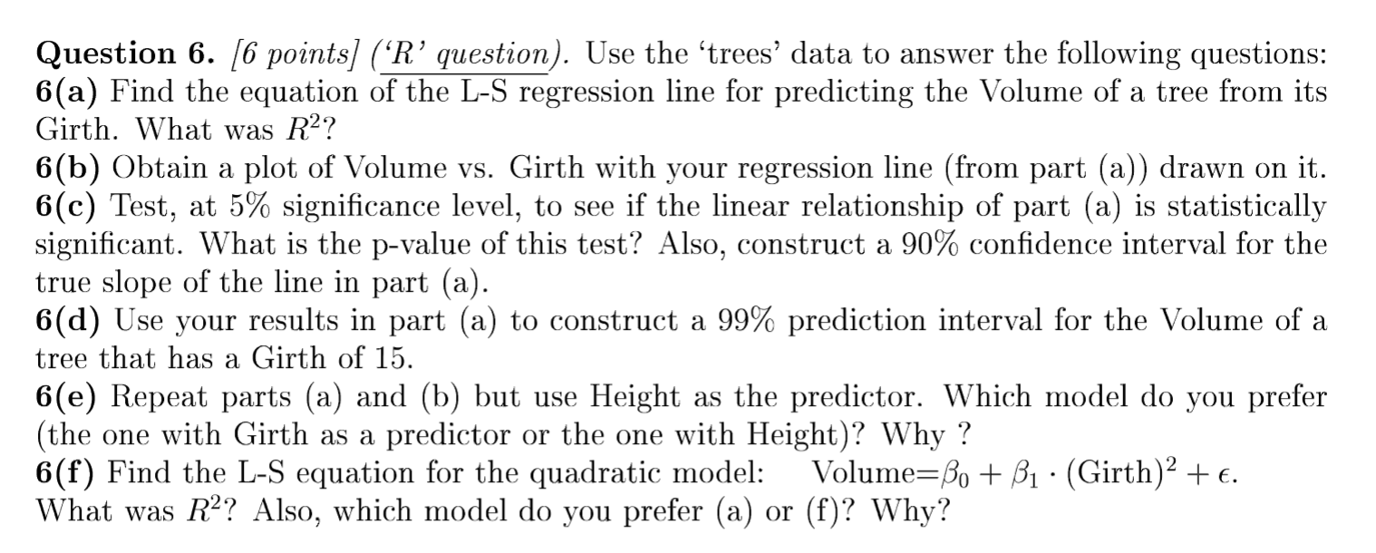
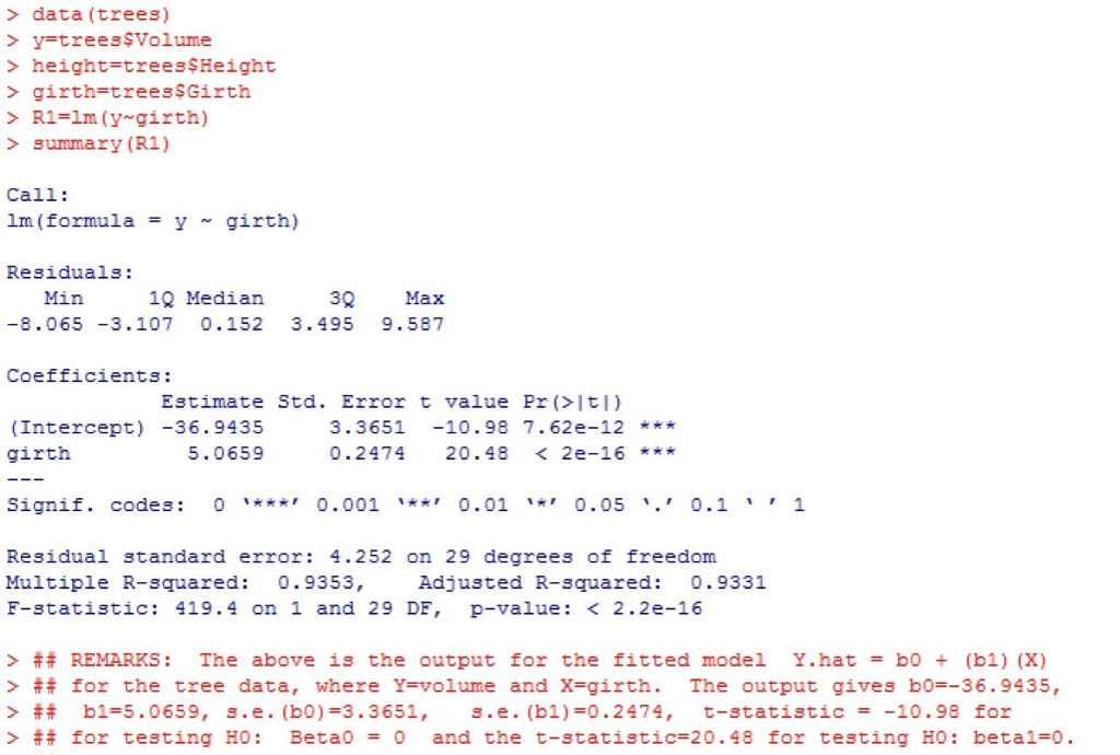
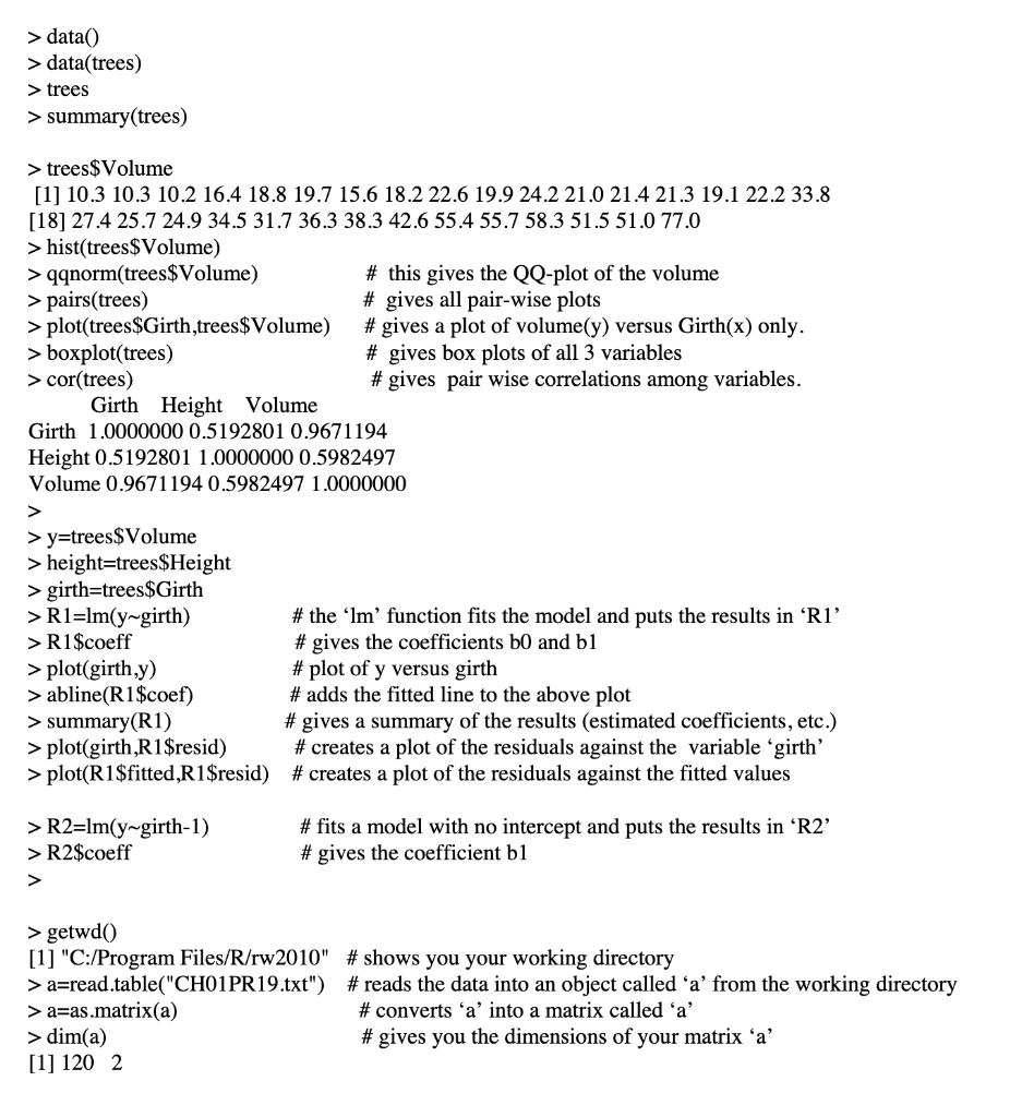
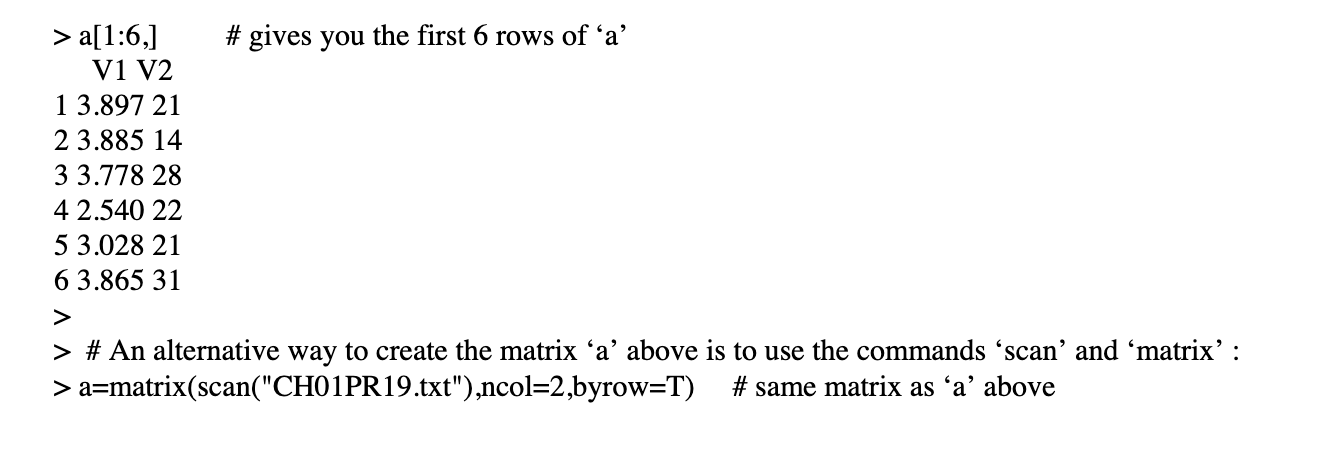
Question 6. [6 points) (R' question). Use the 'trees' data to answer the following questions: 6(a) Find the equation of the L-S regression line for predicting the Volume of a tree from its Girth. What was R? 6(b) Obtain a plot of Volume vs. Girth with your regression line (from part (a)) drawn on it. 6(c) Test, at 5% significance level, to see if the linear relationship of part (a) is statistically significant. What is the p-value of this test? Also, construct a 90% confidence interval for the true slope of the line in part (a). 6(d) Use your results in part (a) to construct a 99% prediction interval for the Volume of a tree that has a Girth of 15. 6(e) Repeat parts (a) and (b) but use Height as the predictor. Which model do you prefer (the one with Girth as a predictor or the one with Height)? Why ? 6(f) Find the L-S equation for the quadratic model: Volume=Bo + B1 (Girth)? + . What was R2? Also, which model do you prefer (a) or (f)? Why? >data (trees) > y=trees Volume > height=treessHeight > girth=treessGirth > Ri=lm (yogirth) > summary (R1) Call: im (formula = y girth) Residuals: Min 10 Median -8.065 -3.107 0.152 30 3.495 Max 9.587 Coefficients: Estimate Std. Error t value Pr(tl) (Intercept) -36.9435 3.3651 -10.98 7.62e-12 *** girth 5.0659 0.2474 20.48 ## REMARKS: The above is the output for the fitted model Y.hat = b0 + (51) (X) > ## for the tree data, where Y=volume and X=girth. The output gives b0=-36.9435, > ## b1=5.0659, 3.e. (b0)=3.3651, 3.e. (61)=0.2474, t-statistic = -10.98 for > ## for testing HO: Beta0 = 0 and the t-statistic=20.48 for testing HO: betal=0. > data) >data(trees) > trees > summary(trees) > trees$Volume [1] 10.3 10.3 10.2 16.4 18.8 19.7 15.6 18.2 22.6 19.9 24.2 21.0 21.4 21.3 19.1 22.2 33.8 [18] 27.4 25.7 24.9 34.5 31.7 36.3 38.3 42.6 55.4 55.7 58.3 51.5 51.0 77.0 > hist(trees $Volume) >qqnorm(trees$Volume) # this gives the QQ-plot of the volume > pairs(trees) # gives all pair-wise plots > plot(trees$Girth,trees $Volume) #gives a plot of volume(y) versus Girth(x) only. > boxplot(trees) # gives box plots of all 3 variables > cor(trees) # gives pair wise correlations among variables. Girth Height Volume Girth 1.0000000 0.5192801 0.9671194 Height 0.5192801 1.0000000 0.5982497 Volume 0.9671194 0.5982497 1.0000000 > y=trees $Volume > height=trees $Height > girth=trees$Girth > R1=lm(y-girth) > R1$coeff > plot(girth,y) > abline(R1$coef) > summary(R1) > plot(girth,R1$resid) > plot(R1$fitted,R 1$resid) # the 'Im' function fits the model and puts the results in R1' #gives the coefficients b0 and b1 # plot of y versus girth # adds the fitted line to the above plot # gives a summary of the results (estimated coefficients, etc.) # creates a plot of the residuals against the variable 'girth' # creates a plot of the residuals against the fitted values > R2=lm(y-girth-1) > R2$coeff # fits a model with no intercept and puts the results in R2' #gives the coefficient b1 >getwd() [1] "C:/Program Files/R/rw 2010" # shows you your working directory > a=read.table("CHO1PR19.txt") # reads the data into an object called 'a' from the working directory > a=as.matrix(a) # converts 'a' into a matrix called 'a' > dim(a) # gives you the dimensions of your matrix 'a' [1] 120 2 #gives you the first 6 rows of 'a' > a[1:6,] V1 V2 1 3.897 21 2 3.885 14 33.778 28 4 2.540 22 5 3.028 21 6 3.865 31 > # An alternative way to create the matrix a above is to use the commands 'scan' and 'matrix': > a=matrix(scan("CH01PR19.txt"),ncol=2,byrow=T) # same matrix as 'a' above Question 6. [6 points) (R' question). Use the 'trees' data to answer the following questions: 6(a) Find the equation of the L-S regression line for predicting the Volume of a tree from its Girth. What was R? 6(b) Obtain a plot of Volume vs. Girth with your regression line (from part (a)) drawn on it. 6(c) Test, at 5% significance level, to see if the linear relationship of part (a) is statistically significant. What is the p-value of this test? Also, construct a 90% confidence interval for the true slope of the line in part (a). 6(d) Use your results in part (a) to construct a 99% prediction interval for the Volume of a tree that has a Girth of 15. 6(e) Repeat parts (a) and (b) but use Height as the predictor. Which model do you prefer (the one with Girth as a predictor or the one with Height)? Why ? 6(f) Find the L-S equation for the quadratic model: Volume=Bo + B1 (Girth)? + . What was R2? Also, which model do you prefer (a) or (f)? Why? >data (trees) > y=trees Volume > height=treessHeight > girth=treessGirth > Ri=lm (yogirth) > summary (R1) Call: im (formula = y girth) Residuals: Min 10 Median -8.065 -3.107 0.152 30 3.495 Max 9.587 Coefficients: Estimate Std. Error t value Pr(tl) (Intercept) -36.9435 3.3651 -10.98 7.62e-12 *** girth 5.0659 0.2474 20.48 ## REMARKS: The above is the output for the fitted model Y.hat = b0 + (51) (X) > ## for the tree data, where Y=volume and X=girth. The output gives b0=-36.9435, > ## b1=5.0659, 3.e. (b0)=3.3651, 3.e. (61)=0.2474, t-statistic = -10.98 for > ## for testing HO: Beta0 = 0 and the t-statistic=20.48 for testing HO: betal=0. > data) >data(trees) > trees > summary(trees) > trees$Volume [1] 10.3 10.3 10.2 16.4 18.8 19.7 15.6 18.2 22.6 19.9 24.2 21.0 21.4 21.3 19.1 22.2 33.8 [18] 27.4 25.7 24.9 34.5 31.7 36.3 38.3 42.6 55.4 55.7 58.3 51.5 51.0 77.0 > hist(trees $Volume) >qqnorm(trees$Volume) # this gives the QQ-plot of the volume > pairs(trees) # gives all pair-wise plots > plot(trees$Girth,trees $Volume) #gives a plot of volume(y) versus Girth(x) only. > boxplot(trees) # gives box plots of all 3 variables > cor(trees) # gives pair wise correlations among variables. Girth Height Volume Girth 1.0000000 0.5192801 0.9671194 Height 0.5192801 1.0000000 0.5982497 Volume 0.9671194 0.5982497 1.0000000 > y=trees $Volume > height=trees $Height > girth=trees$Girth > R1=lm(y-girth) > R1$coeff > plot(girth,y) > abline(R1$coef) > summary(R1) > plot(girth,R1$resid) > plot(R1$fitted,R 1$resid) # the 'Im' function fits the model and puts the results in R1' #gives the coefficients b0 and b1 # plot of y versus girth # adds the fitted line to the above plot # gives a summary of the results (estimated coefficients, etc.) # creates a plot of the residuals against the variable 'girth' # creates a plot of the residuals against the fitted values > R2=lm(y-girth-1) > R2$coeff # fits a model with no intercept and puts the results in R2' #gives the coefficient b1 >getwd() [1] "C:/Program Files/R/rw 2010" # shows you your working directory > a=read.table("CHO1PR19.txt") # reads the data into an object called 'a' from the working directory > a=as.matrix(a) # converts 'a' into a matrix called 'a' > dim(a) # gives you the dimensions of your matrix 'a' [1] 120 2 #gives you the first 6 rows of 'a' > a[1:6,] V1 V2 1 3.897 21 2 3.885 14 33.778 28 4 2.540 22 5 3.028 21 6 3.865 31 > # An alternative way to create the matrix a above is to use the commands 'scan' and 'matrix': > a=matrix(scan("CH01PR19.txt"),ncol=2,byrow=T) # same matrix as 'a' above