Need MAT LAB Help

Original Problem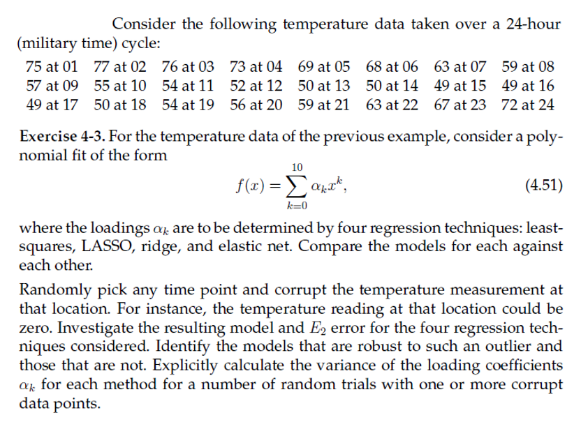

MATLAB CODE

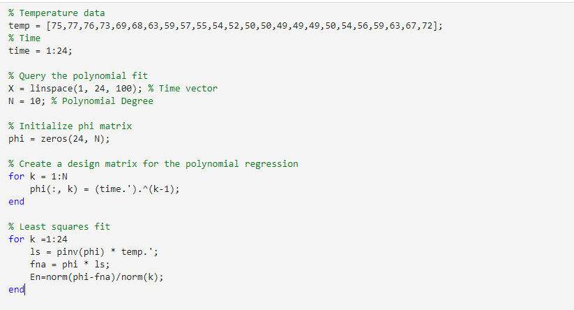
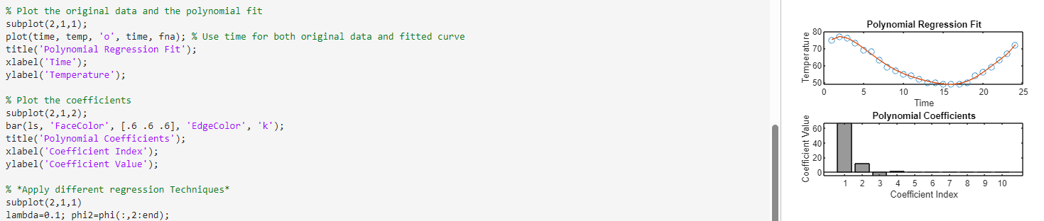
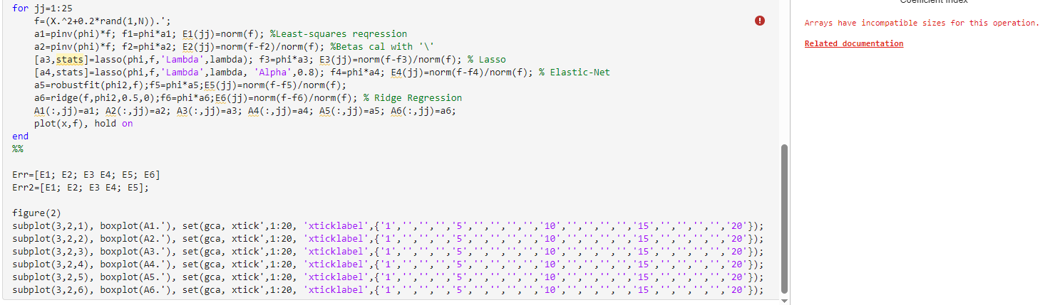
Consider the following temperature data taken over a 24-hour (military time) cycle: \begin{tabular}{llllllll} 75 at 01 & 77 at 02 & 76 at 03 & 73 at 04 & 69 at 05 & 68 at 06 & 63 at 07 & 59 at 08 \\ 57 at 09 & 55 at 10 & 54 at 11 & 52 at 12 & 50 at 13 & 50 at 14 & 49 at 15 & 49 at 16 \\ 49 at 17 & 50 at 18 & 54 at 19 & 56 at 20 & 59 at 21 & 63 at 22 & 67 at 23 & 72 at 24 \end{tabular} Exercise 4-3. For the temperature data of the previous example, consider a polynomial fit of the form f(x)=k=010kxk where the loadings k are to be determined by four regression techniques: leastsquares, LASSO, ridge, and elastic net. Compare the models for each against each other. Randomly pick any time point and corrupt the temperature measurement at that location. For instance, the temperature reading at that location could be zero. Investigate the resulting model and E2 error for the four regression techniques considered. Identify the models that are robust to such an outlier and those that are not. Explicitly calculate the variance of the loading coefficients k for each method for a number of random trials with one or more corrupt data points. \% Temperature data temp =[75,77,76,73,69,68,63,59,57,55,54,52,50,50,49,49,49,50,54,56,59,63,67,72]; % Time time =1:24; \% Query the polynomial fit X= linspace (1,24,100);% Time vector N=10;% Polynomial Degree \% Initialize phi matrix phi =zeros(24,N); \% Create a design matrix for the polynomial regression for k=1:N phi(:, k) =( time. ').^(k-1); end % Least squares fit for k=1:24 ls = pinv(phi) * temp. ' ; fna = phi * 15 ; En=norm(phi-fna)orm(k); end \% Plot the original data and the polynomial fit subplot (2,1,1); plot(time, temp, 'o', time, fna); \% Use time for both original data and fitted curve title('Polynomial Regression Fit'); xlabel('Time'); ylabel( 'Temperature'); \% Plot the coefficients subplot (2,1,2); bar(1s, 'FaceColor', [. . .6.6], 'EdgeColor', 'k'); title('Polynomial Coefficients'); xlabel('Coefficient Index'); ylabel('Coefficient Value'); \% *Apply different regression Techniques* subplot (2,1,1) lambda=0.1; phi2=phi(:,2:end); for jj=1:25 f=(X+0.2rand(1,N)).; a1=pinv(phi)*f; f1= phi*a1; E1(jj)=norm(f); \%Least-squares reqression a2=pinv(phi)*f; f2= phi*a2; E2(jj)=norm(f-f2)orm(f); \%Betas cal with ' \ ' [a3,stats]=lasso(phi,f,' Lambda', lambda); f3= phi*a3; E3(jj)=norm(ff3)/ norm(f); \% Lasso [a4,stats]=lasso(phi,f,'Lambda', lambda, 'Alpha', 0.8); f4= phi*a4; E4(jj)=norm(ff4)/ norm(f); \% Elastic-Net a5=robustfit(phi2,f);f5=phi*a5;E5(jj)=norm(f-f5)orm(f); a6=ridge (f,phi2, .5,0);f6= phi*a6;E6 (jj)=norm(ff6)/ norm (f);% Ridge Regression A1(:,jj)=a1;A2(:,jj)=a2;A3(:,jj)=a3;A4(:,jj)=a4;A5(:,jj)=a5;A6(:,jj)=a6; plot (x,f), hold on end % Err=[E1;E2;E3E4;E5;E6] Err2 =[E1;E2;E3 E4; E5]; figure(2) Arrays have incompatible sizes for this operation. Related documentation