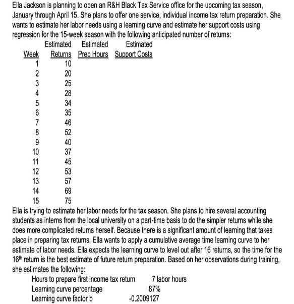
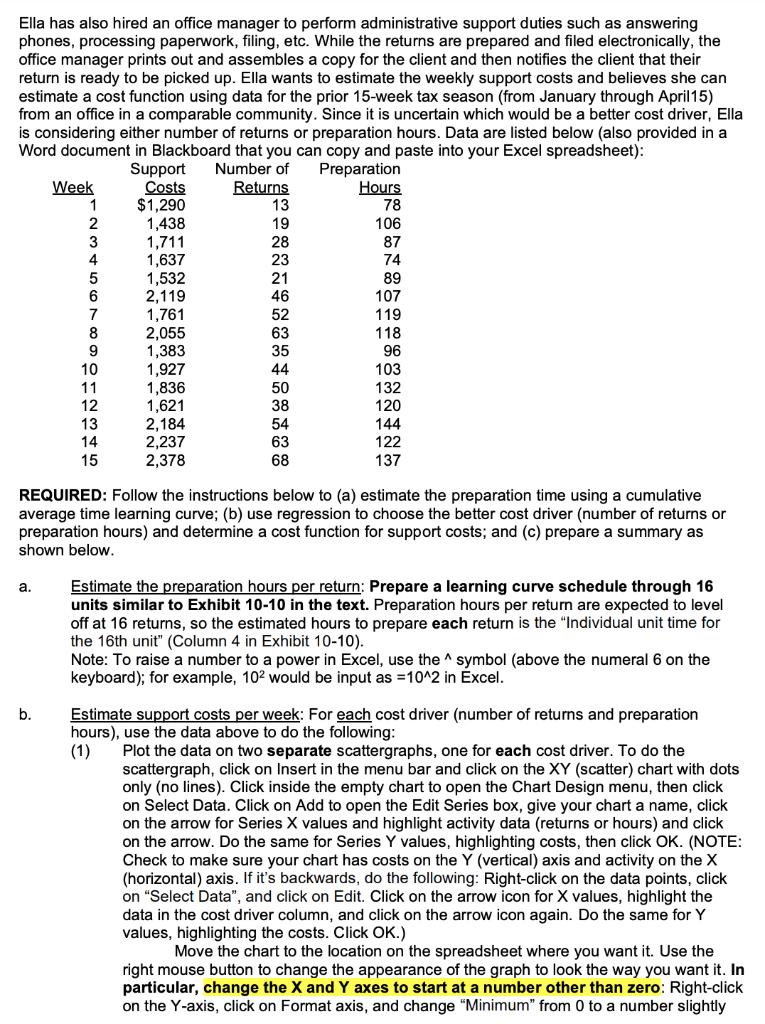
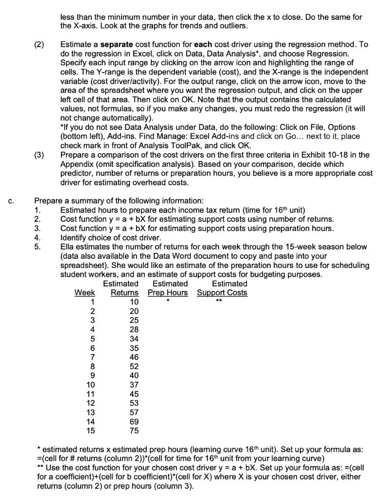
Ella Jackson is planning to open an R&H Black Tax Service office for the upcoming tax season, January through April 15. She plans to offer one service, individual income tax return preparation. She wants to estimate her labor needs using a learning curve and estimate her support costs using regression for the 15-week season with the following anticipated number of returns: Estimated Estimated Estimated Returns Prep Hours Support Costs 10 20 25 Week 1 2 3 4 5 56 6 7 8 9 10 11 28 34 35 46 52 40 37 45 53 57 12 13 14 69 15 75 Ella is trying to estimate her labor needs for the tax season. She plans to hire several accounting students as interns from the local university on a part-time basis to do the simpler returns while she does more complicated returns herself. Because there is a significant amount of learning that takes place in preparing tax returns, Ella wants to apply a cumulative average time learning curve to her estimate of labor needs. Ella expects the learning curve to level out after 16 returns, so the time for the 16th return is the best estimate of future return preparation. Based on her observations during training, she estimates the following: Hours to prepare first income tax return Learning curve percentage Learning curve factor b 7 labor hours 87% -0.2009127 Ella has also hired an office manager to perform administrative support duties such as answering phones, processing paperwork, filing, etc. While the returns are prepared and filed electronically, the office manager prints out and assembles a copy for the client and then notifies the client that their return is ready to be picked up. Ella wants to estimate the weekly support costs and believes she can estimate a cost function using data for the prior 15-week tax season (from January through April15) from an office in a comparable community. Since it is uncertain which would be a better cost driver, Ella is considering either number of returns or preparation hours. Data are listed below (also provided in a Word document in Blackboard that you can copy and paste into your Excel spreadsheet): Number of Preparation Returns 13 19 28 23 21 46 52 Week 1 2 3 4 5 6 7 8 9 10 11 b. 12 13 14 15 Support Costs $1,290 1,438 1,711 1,637 1,532 2,119 1,761 2,055 1,383 1,927 1,836 1,621 2,184 2,237 2,378 63 35 44 50 38 54 63 68 Hours 78 106 87 74 89 107 119 118 96 103 132 120 144 122 137 REQUIRED: Follow the instructions below to (a) estimate the preparation time using a cumulative average time learning curve; (b) use regression to choose the better cost driver (number of returns or preparation hours) and determine a cost function for support costs; and (c) prepare a summary as shown below. a. Estimate the preparation hours per return: Prepare a learning curve schedule through 16 units similar to Exhibit 10-10 in the text. Preparation hours per return are expected to level off at 16 returns, so the estimated hours to prepare each return is the "Individual unit time for the 16th unit" (Column 4 in Exhibit 10-10). Note: To raise a number to a power in Excel, use the symbol (above the numeral 6 on the keyboard); for example, 102 would be input as = 10^2 in Excel. Estimate support costs per week: For each cost driver (number of returns and preparation hours), use the data above to do the following: (1) Plot the data on two separate scattergraphs, one for each cost driver. To do the scattergraph, click on Insert in the menu bar and click on the XY (scatter) chart with dots only (no lines). Click inside the empty chart to open the Chart Design menu, then click on Select Data. Click on Add to open the Edit Series box, give your chart a name, click on the arrow for Series X values and highlight activity data (returns or hours) and click on the arrow. Do the same for Series Y values, highlighting costs, then click OK. (NOTE: Check to make sure your chart has costs on the Y (vertical) axis and activity on the X (horizontal) axis. If it's backwards, do the following: Right-click on the data points, click on "Select Data", and click on Edit. Click on the arrow icon for X values, highlight the data in the cost driver column, and click on the arrow icon again. Do the same for Y values, highlighting the costs. Click OK.) Move the chart to the location on the spreadsheet where you want it. Use the right mouse button to change the appearance of the graph to look the way you want it. In particular, change the X and Y axes to start at a number other than zero: Right-click on the Y-axis, click on Format axis, and change "Minimum" from 0 to a number slightly C. (2) (3) 123410 less than the minimum number in your data, then click the x to close. Do the same for the X-axis. Look at the graphs for trends and outliers. 1. 2. 3. Estimate a separate cost function for each cost driver using the regression method. To do the regression in Excel, click on Data, Data Analysis*, and choose Regression. Specify each input range by clicking on the arrow icon and highlighting the range of cells. The Y-range is the dependent variable (cost), and the X-range is the independent variable (cost driver/activity). For the output range, click on the arrow icon, move to the area of the spreadsheet where you want the regression output, and click on the upper left cell of that area. Then click on OK. Note that the output contains the calculated values, not formulas, so if you make any changes, you must redo the regression (it will not change automatically). Prepare a summary of the following information: 5. *If you do not see Data Analysis under Data, do the following: Click on File, Options (bottom left), Add-ins. Find Manage: Excel Add-ins and click on Go... next to it, place check mark in front of Analysis ToolPak, and click OK. Prepare a comparison of the cost drivers on the first three criteria in Exhibit 10-18 in the Appendix (omit specification analysis). Based on your comparison, decide which Estimated hours to prepare each income tax return (time for 16th unit) Cost function y = a + bX for estimating support costs using number of returns. Cost function y = a + bX for estimating support costs using preparation hours. 4. Identify choice of cost driver. predictor, number of returns or preparation hours, you believe is a more appropriate cost driver for estimating overhead costs. Ella estimates the number of returns for each week through the 15-week season below (data also available in the Data Word document to copy and paste into your spreadsheet). She would like an estimate of the preparation hours to use for scheduling student workers, and an estimate of support costs for budgeting purposes. Estimated Support Costs Week 1 2 3 4 5 6 7 8 9 SO123H5 10 11 14 Estimated Estimated Returns Prep Hours 10 20 25 28 34 35 46 52 40 37 45 53 57 69 75 * ** * estimated returns x estimated prep hours (learning curve 16th unit). Set up your formula as: =(cell for # returns (column 2))*(cell for time for 16th unit from your learning curve) ** Use the cost function for your chosen cost driver y = a + bX. Set up your formula as: =(cell for a coefficient)+(cell for b coefficient)*(cell for X) where X is your chosen cost driver, either returns (column 2) or prep hours (column 3).