Normal Curve Areas P(z < 1.23) = Area 0.8907 Z 0.02 0 1.23 0.04 0.0003 0.05...

Transcribed Image Text:

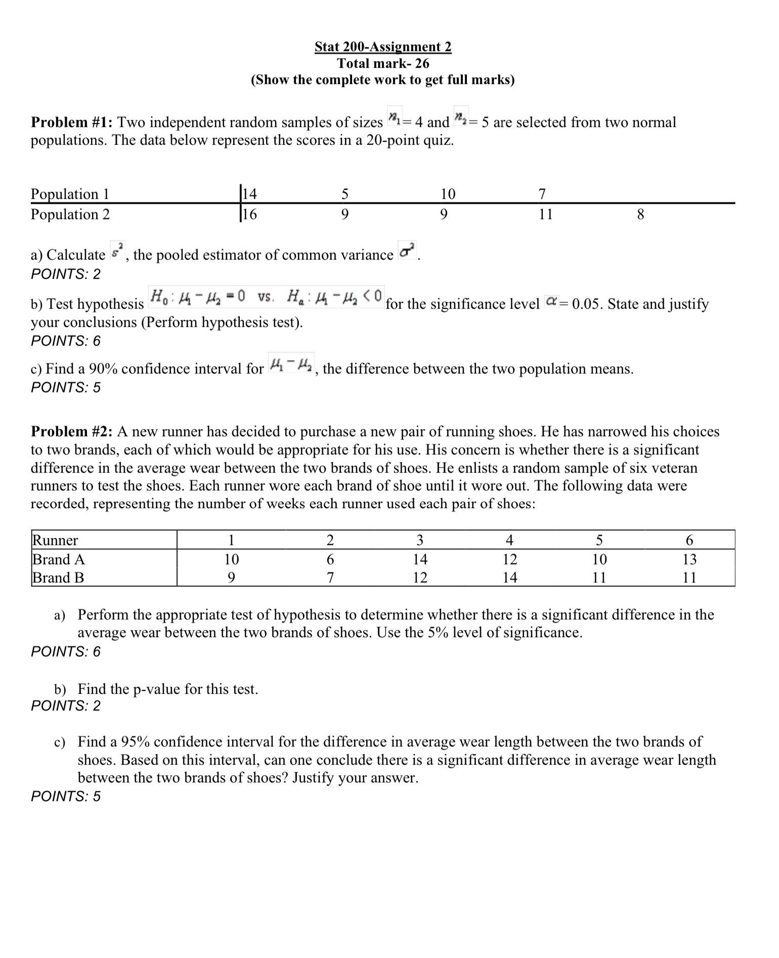
Normal Curve Areas P(z < 1.23) = Area 0.8907 Z 0.02 0 1.23 0.04 0.0003 0.05 0.06 2 0.00 0.01 0.03 0.07 0.08 0.09 -3.4 0.0003 0.0003 0.0003 0.0003 0.0003 0.0003 0.0003 0.0003 0.0002 -3.3 0.0005 0.0005 0.0005 0.0004 0.0004 0.0004 0.0004 0.0004 0.0004 0.0003 -3.2 0.0007 0.0007 0.0006 0.0006 0.0006 0.0006 0.0006 0.0005 0.0005 0.0005 -3.1 0.0010 0.0009 0.0009 0.0009 0.0008 0.0008 0.0008 0.0008 0.0007 0.0007 -3.0 0.0013 0.0013 0.0013 0.0012 0.0012 0.0011 0.0011 0.0011 0.0010 0.0010 -2.9 0.0019 0.0018 0.0018 0.0017 0.0016 0.0016 0.0015 0.0015 0.0014 0.0014 -2.8 0.0026 0.0025 0.0024 0.0023 0.0023 0.0022 0.0021 0.0021 0.0020 0.0019 -2.7 0.0035 0.0034 0.0033 0.0032 0.0031 0.0030 0.0029 0.0028 0.0027 0.0026 -2.6 0.0047 0.0045 0.0044 0.0043 0.0041 0.0040 0.0039 0.0038 0.0037 0.0036 -2.5 0.0062 0.0060 0.0059 0.0057 0.0055 0.0054 0.0052 0.0051 0.0049 0.0048 -2.4 0.0082 0.0080 0.0078 0.0075 0.0073 0.0071 0.0069 0.0068 0.0066 0.0064 -2.3 0.0107 0.0104 0.0102 0.0099 0.0096 0.0094 0.0091 0.0089 0.0087 0.0084 -2.2 0.0139 0.0136 0.0132 0.0129 0.0125 0.0122 0.0119 0.0116 0.0113 0.0110 -2.1 0.0179 0.0174 0.0170 0.0166 0.0162 0.0158 0.0154 0.0150 0.0146 0.0143 -2.0 0.0228 0.0222 0.0217 0.0212 0.0207 0.0202 0.0197 0.0192 0.0188 0.0183 -1.9 0.0287 0.0281 0.0274 0.0268 0.0262 0.0256 0.0250 0.0244 0.0239 0.0233 -1.8 0.0359 0.0351 0.0344 0.0336 0.0329 0.0322 0.0314 0.0307 0.0301 0.0294 -1.7 0.0446 0.0436 0.0427 0.0418 0.0409 0.0401 0.0392 0.0384 0.0375 0.0367 -1.6 0.0548 0.0537 0.0526 0.0516 0.0505 0.0495 0.0485 0.0475 0.0465 0.0455 -1.5 0.0668 0.0655 0.0643 0.0630 0.0618 0.0606 0.0594 0.0582 0.0571 0.0559 -1.4 0.0808 0.0793 0.0778 0.0764 0.0749 0.0735 0.0721 0.0708 0.0694 0.0681 -1.3 0.0968 0.0951 0.0934 0.0918 0.0901 0.0885 0.0869 0.0853 0.0838 0.0823 -1.2 0.1151 0.1131 0.1112 0.1093 0.1075 0.1056 0.1038 0.1020 0.1003 0.0985 -1.1 0.1357 0.1335 0.1314 0.1292 0.1271 0.1251 0.1230 0.1210 0.1190 0.1170 -1.0 0.1587 0.1562 0.1539 0.1515 0.1492 0.1469 0.1446 0.1423 0.1401 0.1379 -0.9 0.1841 0.1814 0.1788 0.1762 0.1736 0.1711 0.1685 0.1660 0.1635 0.1611 -0.8 0.2119 0.2090 0.2061 0.2033 0.2005 0.1977 0.1949 0.1922 0.1894 0.1867 -0.7 0.2420 0.2389 0.2358 0.2327 0.2296 0.2266 0.2236 0.2206 0.2177 0.2148 -0.6 0.2743 0.2709 0.2676 0.2643 0.2611 0.2578 0.2546 0.2514 0.2483 0.2451 -0.5 0.3085 0.3050 0.3015 0.2981 0.2946 0.2912 0.2877 0.2843 0.2810 0.2776 -0.4 0.3446 0.3409 0.3372 0.3336 0.3300 0.3264 0.3228 0.3192 0.3156 0.3121 -0.3 0.3821 0.3783 0.3745 0.3707 0.3669 0.3632 0.3594 0.3557 0.3520 0.3483 -0.2 0.4207 0.4168 0.4129 0.4090 0.4052 0.4013 0.3974 0.3936 0.3897 0.3859 -0.1 0.4602 0.4562 0.4522 0.4483 0.4443 0.4404 0.4364 0.4325 0.4286 0.4247 -0.0 0.5000 0.4960 0.4920 0.4880 0.4840 0.4801 0.4761 0.4721 0.4681 0.4641 2 0.00 0.03 0.04 0.05 0.06 0.07 0.08 0.01 0.02 0.09 0.0 0.5000 0.5040 0.5080 0.5120 0.5160 0.5199 0.5239 0.5279 0.5319 0.5359 0.1 0.5398 0.5438 0.5478 0.5517 0.5557 0.5596 0.5636 0.5675 0.5714 0.5753 0.2 0.5793 0.5832 0.5871 0.5910 0.5948 0.5987 0.6026 0.6064 0.6103 0.6141 0.3 0.6179 0.6217 0.6255 0.6293 0.6331 0.6368 0.6406 0.6443 0.6480 0.6517 0.4 0.6554 0.6591 0.6628 0.6664 0.6700 0.6736 0.6772 0.6808 0.6844 0.6879 0.5 0.6915 0.6950 0.6985 0.7019 0.7054 0.7088 0.7123 0.7157 0.7190 0.7224 0.6 0.7257 0.7291 0.7324 0.7357 0.7389 0.7422 0.7454 0.7486 0.7517 0.7549 0.7 0.7580 0.7611 0.7642 0.7673 0.7704 0.7734 0.7764 0.7794 0.7823 0.7852 0.8 0.7881 0.7910 0.7939 0.7967 0.7995 0.8023 0.8051 0.8078 0.8106 0.8133 0.9 0.8159 0.8186 0.8212 0.8238 0.8264 0.8289 0.8315 0.8340 0.8365 0.8389 1.0 0.8413 0.8438 0.8461 0.8485 0.8508 0.8531 0.8554 0.8577 0.8599 0.8621 1.1 0.8643 0.8665 0.8686 0.8708 0.8729 0.8749 0.8770 0.8790 0.8810 0.8830 0.8849 0.8869 0.8888 0.8907 0.8925 0.8944 0.8962 0.8980 0.8997 0.9015 1.3 0.9032 0.9049 0.9066 0.9082 0.9099 0.9115 0.9131 0.9147 0.9162 0.9177 1.4 0.9192 0.9207 0.9222 0.9236 0.9251 0.9265 0.9279 0.9292 0.9306 0.9319 1.2 1.5 0.9332 0.9345 0.9357 0.9370 0.9382 0.9394 0.9406 0.9418 0.9429 0.9441 1.6 0.9452 0.9463 0.9474 0.9484 0.9495 0.9505 0.9515 0.9525 0.9535 0.9545 1.7 0.9554 0.9564 0.9573 0.9582 0.9591 0.9599 0.9608 0.9616 0.9625 0.9633 1.8 0.9641 0.9649 0.9656 0.9664 0.9671 0.9678 0.9686 0.9693 0.9699 0.9706 1.9 0.9713 0.9719 0.9726 0.9732 0.9738 0.9744 0.9750 0.9756 0.9761 0.9767 2.0 0.9772 0.9778 0.9783 0.9788 0.9793 0.9798 0.9803 0.9808 0.9812 0.9817 2.1 0.9821 0.9826 0.9830 0.9834 0.9838 0.9842 0.9846 0.9850 0.9854 0.9857 2.2 0.9861 0.9864 0.9868 0.9871 0.9875 0.9878 0.9881 0.9884 0.9887 0.9890 2.3 0.9893 0.9896 0.9898 0.9901 0.9901 0.9906 0.9909 0.9911 0.9913 0.9916 2.4 0.9918 0.9920 0.9922 0.9925 0.9927 0.9929 0.9931 0.9932 0.9934 0.9936 2.5 0.9938 0.9940 0.9941 0.9943 0.9945 0.9946 0.9948 0.9949 0.9951 0.9952 2.6 0.9953 0.9955 0.9956 0.9957 0.9959 0.9960 0.9961 0.9962 0.9963 0.9964 2.7 0.9965 0.9966 0.9967 0.9968 0.9969 0.9970 0.9971 0.9972 0.9973 0.9974 2.8 0.9974 0.9975 0.9976 0.9977 0.9977 0.9978 0.9979 0.9979 0.9980 0.9981 2.9 0.9981 0.9982 0.9982 0.9983 0.9984 0.9984 0.9985 0.9985 0.9986 0.9986 3.0 0.9987 0.9987 0.9987 0.9988 0.9988 0.9989 0.9989 0.9989 0.9990 0.9990 3.1 0.9990 0.9991 0.9991 0.9991 0.9992 0.9992 0.9992 0.9992 0.9993 0.9993 3.2 0.9993 0.9993 0.9994 0.9994 0.9994 0.9994 0.9994 0.9995 0.9995 0.9995 3.3 0.9995 0.9995 0.9995 0.9996 0.9996 0.9996 0.9996 0.9996 0.9996 0.9997 3.4 0.9997 0.9997 0.9997 0.9997 0.9997 0.9997 0.9997 0.9997 0.9997 0.9998 Student's t Distribution (Critical Values) 1- a -t t Left-tailed Test Right-tailed Test -t Two-tailed Test t t -t Confidence Interval Confidence Coefficient, 1-a 0.80 0.90 df 0.95 Level of Significance for One-Tailed Test, a 0.100 0.050 0.025 0.010 0.005 0.98 0.99 0.999 df 0.0005 Level of Significance for Two-Tailed Test, a Confidence Coefficient, 1-a 0.80 0.90 0.95 0.98 0.99 0.999 Level of Significance for One-Tailed Test, a 0.100 0.050 0.025 0.010 0.005 0.0005 Level of Significance for Two-Tailed Test, a 0.20 0.10 0.05 0.02 0.01 0.001 0.20 0.10 0.05 0.02 0.01 0.001 12315 3.078 6.314 12.706 31.821 63.657 1.886 2.920 4.303 6.965 9.925 1.638 2.353 3.182 4.541 5.841 1.533 2.132 2.776 3.747 4.604 1.476 2.015 2.571 3.365 4.032 636.619 31.599 12.924 31 32 33 1.308 1.309 1.696 2.040 2.453 2.744 3.633 1.309 1.694 2.037 2.449 2.738 3.622 1.692 2.035 2.445 2.733 3.611 8.610 34 1.307 1.691 2.032 2.441 2.728 3.601 6.869 35 1.306 1.690 2.030 2.438 2.724 3.591 08129 6 1.440 1.943 2.447 3.143 3.707 5.959 36 1.306 1.688 2.028 2.434 2.719 3.582 7 1.415 1.895 2.365 1.397 1.860 2.306 2.896 1.383 1.833 2.262 2.821 1.372 1.812 2.228 2.764 2.998 3.499 5.408 37 1.305 1.687 2.026 2.431 2.715 3.574 3.355 5.041 38 1.304 1.686 2.024 2.429 2.712 3.566 3.250 4.781 39 3.169 4.587 40 1.304 1.303 1.685 2.023 2.426 2.708 1.684 2.021 2.423 2.704 3.558 3.551 11 1.363 1.796 2.201 2.718 3.106 4.437 12 1.356 1.782 2.179 2.681 3.055 4.318 42 13 1.350 1.771 2.160 2.650 3.012 4.221 43 14 1.345 1.761 15 1.341 1.753 2.145 2.131 2.624 2.977 2.602 2.947 4.140 4.073 12345 41 1.303 1.683 2.020 2.421 2.701 1.302 1.682 2.018 2.418 2.698 1.302 1.681 2.017 2.416 2.695 3.544 3.538 3.532 44 1.301 1.680 2.015 2.414 2.692 45 1.301 1.679 2.014 2.412 2.690 3.526 3.520 STLOO 20 1.325 1.725 16 1.337 1.746 2.120 2.583 2.921 17 1.333 1.740 2.110 2.567 2.898 18 1.330 1.734 2.101 2.552 2.878 19 1.328 1.729 2.093 2.086 4.015 3.965 3.922 2.539 2.861 2.528 2.845 3.883 3.850 9149 46 1.300 1.679 2.013 2.410 2.687 3.515 47 1.300 1.678 2.012 2.408 2.685 3.510 48 1.299 1.677 2.011 2.407 2.682 3.505 49 1.299 1.677 2.010 2.405 2.680 3.500 50 1.299 1.676 2.009 2.403 2.678 3.496 21 1.323 1.721 2.080 2.518 223 22 1.321 1.717 2.074 2.508 23 1.319 1.714 2.069 2.500 2.807 2.831 2.819 3.819 51 3.792 3.768 24 1.318 1.711 25 1.316 1.708 2.064 2.492 2.060 2.485 2.797 2.787 3.745 3.725 1.298 1.675 2.008 2.402 2.676 3.492 52 1.298 1.675 2.007 2.400 2.674 3.488 53 1.298 1.674 2.005 2.399 54 1.297 1.674 2.005 2.397 55 1.297 1.673 2.004 2.396 2.668 3.476 2.672 3.484 2.670 3.480 2222 26 27 1.315 1.706 2.056 2.479 2.779 1.314. 1.703 2.052 2.473 2.771 28 1.313 1.701 2.048 2.467 2.763 29 1.311 1.699 2.045 2.462 2.756 30 1.310 1.697 2.042 2.457 2.750 3.707 3.690 3.674 3.659 3.646 60 1.296 1.671 2.000 2.390 2.660 3.460 80 1.292 1.664 1.990 2.374 2.639 3.416 100 1.290 1.660 1.984 2.364 2.626 3.390 200 1.286 1.653 1.972 2.345 2.601 3.340 1.282 1.645 1.960 2.326 2.576 3.291 Stat 200-Assignment 2 Total mark- 26 (Show the complete work to get full marks) 1= Problem #1: Two independent random samples of sizes = 4 and 2 = 5 are selected from two normal populations. The data below represent the scores in a 20-point quiz. Population 1 Population 2 14 5 9 10 9 7 11 8 = Hoth 20 vs. Hath-H <0. for the significance level a = 0.05. State and justify a) Calculate s, the pooled estimator of common variance & POINTS: 2 b) Test hypothesis your conclusions (Perform hypothesis test). POINTS: 6 c) Find a 90% confidence interval for t, the difference between the two population means. POINTS: 5 Problem #2: A new runner has decided to purchase a new pair of running shoes. He has narrowed his choices to two brands, each of which would be appropriate for his use. His concern is whether there is a significant difference in the average wear between the two brands of shoes. He enlists a random sample of six veteran runners to test the shoes. Each runner wore each brand of shoe until it wore out. The following data were recorded, representing the number of weeks each runner used each pair of shoes: Runner Brand A Brand B 1 2 3 4 5 6 10 6 14 12 10 13 9 7 12 14 11 11 a) Perform the appropriate test of hypothesis to determine whether there is a significant difference in the average wear between the two brands of shoes. Use the 5% level of significance. POINTS: 6 b) Find the p-value for this test. POINTS: 2 c) Find a 95% confidence interval for the difference in average wear length between the two brands of shoes. Based on this interval, can one conclude there is a significant difference in average wear length between the two brands of shoes? Justify your answer. POINTS: 5 COMPARING TWO POPULATION MEANS STEPS OF A HYPOTHESIS TEST: Null hypothesis: Ho: = Alternative hypothesis: Two Tailed Test: Ha: H1 H2 One Tailed Test: > 2 (or, Ha ta/2 or t ta (or t < ta when the alternative hypothesis is Ha < 2) or when p value THE PAIRED-Difference TEST OF Null hypothesis: Ho: pd = 0 Alternative hypothesis: HYPOTHESIS Two Tailed Test: Ha: pd #0 One Tailed Test: d>0 (or, Had < 0) d Test Statistic: t = where n = Number of paired differences d = Mean of the sample differences Sa = Standard deviation of the sample differences Rejection region: Reject Ho when Two Tailed Test: t>ta/2 or t ta (or t < -ta when the alternative hypothesis is Had < 0), based on (n-1) degrees of freedom or when p-value Normal Curve Areas P(z < 1.23) = Area 0.8907 Z 0.02 0 1.23 0.04 0.0003 0.05 0.06 2 0.00 0.01 0.03 0.07 0.08 0.09 -3.4 0.0003 0.0003 0.0003 0.0003 0.0003 0.0003 0.0003 0.0003 0.0002 -3.3 0.0005 0.0005 0.0005 0.0004 0.0004 0.0004 0.0004 0.0004 0.0004 0.0003 -3.2 0.0007 0.0007 0.0006 0.0006 0.0006 0.0006 0.0006 0.0005 0.0005 0.0005 -3.1 0.0010 0.0009 0.0009 0.0009 0.0008 0.0008 0.0008 0.0008 0.0007 0.0007 -3.0 0.0013 0.0013 0.0013 0.0012 0.0012 0.0011 0.0011 0.0011 0.0010 0.0010 -2.9 0.0019 0.0018 0.0018 0.0017 0.0016 0.0016 0.0015 0.0015 0.0014 0.0014 -2.8 0.0026 0.0025 0.0024 0.0023 0.0023 0.0022 0.0021 0.0021 0.0020 0.0019 -2.7 0.0035 0.0034 0.0033 0.0032 0.0031 0.0030 0.0029 0.0028 0.0027 0.0026 -2.6 0.0047 0.0045 0.0044 0.0043 0.0041 0.0040 0.0039 0.0038 0.0037 0.0036 -2.5 0.0062 0.0060 0.0059 0.0057 0.0055 0.0054 0.0052 0.0051 0.0049 0.0048 -2.4 0.0082 0.0080 0.0078 0.0075 0.0073 0.0071 0.0069 0.0068 0.0066 0.0064 -2.3 0.0107 0.0104 0.0102 0.0099 0.0096 0.0094 0.0091 0.0089 0.0087 0.0084 -2.2 0.0139 0.0136 0.0132 0.0129 0.0125 0.0122 0.0119 0.0116 0.0113 0.0110 -2.1 0.0179 0.0174 0.0170 0.0166 0.0162 0.0158 0.0154 0.0150 0.0146 0.0143 -2.0 0.0228 0.0222 0.0217 0.0212 0.0207 0.0202 0.0197 0.0192 0.0188 0.0183 -1.9 0.0287 0.0281 0.0274 0.0268 0.0262 0.0256 0.0250 0.0244 0.0239 0.0233 -1.8 0.0359 0.0351 0.0344 0.0336 0.0329 0.0322 0.0314 0.0307 0.0301 0.0294 -1.7 0.0446 0.0436 0.0427 0.0418 0.0409 0.0401 0.0392 0.0384 0.0375 0.0367 -1.6 0.0548 0.0537 0.0526 0.0516 0.0505 0.0495 0.0485 0.0475 0.0465 0.0455 -1.5 0.0668 0.0655 0.0643 0.0630 0.0618 0.0606 0.0594 0.0582 0.0571 0.0559 -1.4 0.0808 0.0793 0.0778 0.0764 0.0749 0.0735 0.0721 0.0708 0.0694 0.0681 -1.3 0.0968 0.0951 0.0934 0.0918 0.0901 0.0885 0.0869 0.0853 0.0838 0.0823 -1.2 0.1151 0.1131 0.1112 0.1093 0.1075 0.1056 0.1038 0.1020 0.1003 0.0985 -1.1 0.1357 0.1335 0.1314 0.1292 0.1271 0.1251 0.1230 0.1210 0.1190 0.1170 -1.0 0.1587 0.1562 0.1539 0.1515 0.1492 0.1469 0.1446 0.1423 0.1401 0.1379 -0.9 0.1841 0.1814 0.1788 0.1762 0.1736 0.1711 0.1685 0.1660 0.1635 0.1611 -0.8 0.2119 0.2090 0.2061 0.2033 0.2005 0.1977 0.1949 0.1922 0.1894 0.1867 -0.7 0.2420 0.2389 0.2358 0.2327 0.2296 0.2266 0.2236 0.2206 0.2177 0.2148 -0.6 0.2743 0.2709 0.2676 0.2643 0.2611 0.2578 0.2546 0.2514 0.2483 0.2451 -0.5 0.3085 0.3050 0.3015 0.2981 0.2946 0.2912 0.2877 0.2843 0.2810 0.2776 -0.4 0.3446 0.3409 0.3372 0.3336 0.3300 0.3264 0.3228 0.3192 0.3156 0.3121 -0.3 0.3821 0.3783 0.3745 0.3707 0.3669 0.3632 0.3594 0.3557 0.3520 0.3483 -0.2 0.4207 0.4168 0.4129 0.4090 0.4052 0.4013 0.3974 0.3936 0.3897 0.3859 -0.1 0.4602 0.4562 0.4522 0.4483 0.4443 0.4404 0.4364 0.4325 0.4286 0.4247 -0.0 0.5000 0.4960 0.4920 0.4880 0.4840 0.4801 0.4761 0.4721 0.4681 0.4641 2 0.00 0.03 0.04 0.05 0.06 0.07 0.08 0.01 0.02 0.09 0.0 0.5000 0.5040 0.5080 0.5120 0.5160 0.5199 0.5239 0.5279 0.5319 0.5359 0.1 0.5398 0.5438 0.5478 0.5517 0.5557 0.5596 0.5636 0.5675 0.5714 0.5753 0.2 0.5793 0.5832 0.5871 0.5910 0.5948 0.5987 0.6026 0.6064 0.6103 0.6141 0.3 0.6179 0.6217 0.6255 0.6293 0.6331 0.6368 0.6406 0.6443 0.6480 0.6517 0.4 0.6554 0.6591 0.6628 0.6664 0.6700 0.6736 0.6772 0.6808 0.6844 0.6879 0.5 0.6915 0.6950 0.6985 0.7019 0.7054 0.7088 0.7123 0.7157 0.7190 0.7224 0.6 0.7257 0.7291 0.7324 0.7357 0.7389 0.7422 0.7454 0.7486 0.7517 0.7549 0.7 0.7580 0.7611 0.7642 0.7673 0.7704 0.7734 0.7764 0.7794 0.7823 0.7852 0.8 0.7881 0.7910 0.7939 0.7967 0.7995 0.8023 0.8051 0.8078 0.8106 0.8133 0.9 0.8159 0.8186 0.8212 0.8238 0.8264 0.8289 0.8315 0.8340 0.8365 0.8389 1.0 0.8413 0.8438 0.8461 0.8485 0.8508 0.8531 0.8554 0.8577 0.8599 0.8621 1.1 0.8643 0.8665 0.8686 0.8708 0.8729 0.8749 0.8770 0.8790 0.8810 0.8830 0.8849 0.8869 0.8888 0.8907 0.8925 0.8944 0.8962 0.8980 0.8997 0.9015 1.3 0.9032 0.9049 0.9066 0.9082 0.9099 0.9115 0.9131 0.9147 0.9162 0.9177 1.4 0.9192 0.9207 0.9222 0.9236 0.9251 0.9265 0.9279 0.9292 0.9306 0.9319 1.2 1.5 0.9332 0.9345 0.9357 0.9370 0.9382 0.9394 0.9406 0.9418 0.9429 0.9441 1.6 0.9452 0.9463 0.9474 0.9484 0.9495 0.9505 0.9515 0.9525 0.9535 0.9545 1.7 0.9554 0.9564 0.9573 0.9582 0.9591 0.9599 0.9608 0.9616 0.9625 0.9633 1.8 0.9641 0.9649 0.9656 0.9664 0.9671 0.9678 0.9686 0.9693 0.9699 0.9706 1.9 0.9713 0.9719 0.9726 0.9732 0.9738 0.9744 0.9750 0.9756 0.9761 0.9767 2.0 0.9772 0.9778 0.9783 0.9788 0.9793 0.9798 0.9803 0.9808 0.9812 0.9817 2.1 0.9821 0.9826 0.9830 0.9834 0.9838 0.9842 0.9846 0.9850 0.9854 0.9857 2.2 0.9861 0.9864 0.9868 0.9871 0.9875 0.9878 0.9881 0.9884 0.9887 0.9890 2.3 0.9893 0.9896 0.9898 0.9901 0.9901 0.9906 0.9909 0.9911 0.9913 0.9916 2.4 0.9918 0.9920 0.9922 0.9925 0.9927 0.9929 0.9931 0.9932 0.9934 0.9936 2.5 0.9938 0.9940 0.9941 0.9943 0.9945 0.9946 0.9948 0.9949 0.9951 0.9952 2.6 0.9953 0.9955 0.9956 0.9957 0.9959 0.9960 0.9961 0.9962 0.9963 0.9964 2.7 0.9965 0.9966 0.9967 0.9968 0.9969 0.9970 0.9971 0.9972 0.9973 0.9974 2.8 0.9974 0.9975 0.9976 0.9977 0.9977 0.9978 0.9979 0.9979 0.9980 0.9981 2.9 0.9981 0.9982 0.9982 0.9983 0.9984 0.9984 0.9985 0.9985 0.9986 0.9986 3.0 0.9987 0.9987 0.9987 0.9988 0.9988 0.9989 0.9989 0.9989 0.9990 0.9990 3.1 0.9990 0.9991 0.9991 0.9991 0.9992 0.9992 0.9992 0.9992 0.9993 0.9993 3.2 0.9993 0.9993 0.9994 0.9994 0.9994 0.9994 0.9994 0.9995 0.9995 0.9995 3.3 0.9995 0.9995 0.9995 0.9996 0.9996 0.9996 0.9996 0.9996 0.9996 0.9997 3.4 0.9997 0.9997 0.9997 0.9997 0.9997 0.9997 0.9997 0.9997 0.9997 0.9998 Student's t Distribution (Critical Values) 1- a -t t Left-tailed Test Right-tailed Test -t Two-tailed Test t t -t Confidence Interval Confidence Coefficient, 1-a 0.80 0.90 df 0.95 Level of Significance for One-Tailed Test, a 0.100 0.050 0.025 0.010 0.005 0.98 0.99 0.999 df 0.0005 Level of Significance for Two-Tailed Test, a Confidence Coefficient, 1-a 0.80 0.90 0.95 0.98 0.99 0.999 Level of Significance for One-Tailed Test, a 0.100 0.050 0.025 0.010 0.005 0.0005 Level of Significance for Two-Tailed Test, a 0.20 0.10 0.05 0.02 0.01 0.001 0.20 0.10 0.05 0.02 0.01 0.001 12315 3.078 6.314 12.706 31.821 63.657 1.886 2.920 4.303 6.965 9.925 1.638 2.353 3.182 4.541 5.841 1.533 2.132 2.776 3.747 4.604 1.476 2.015 2.571 3.365 4.032 636.619 31.599 12.924 31 32 33 1.308 1.309 1.696 2.040 2.453 2.744 3.633 1.309 1.694 2.037 2.449 2.738 3.622 1.692 2.035 2.445 2.733 3.611 8.610 34 1.307 1.691 2.032 2.441 2.728 3.601 6.869 35 1.306 1.690 2.030 2.438 2.724 3.591 08129 6 1.440 1.943 2.447 3.143 3.707 5.959 36 1.306 1.688 2.028 2.434 2.719 3.582 7 1.415 1.895 2.365 1.397 1.860 2.306 2.896 1.383 1.833 2.262 2.821 1.372 1.812 2.228 2.764 2.998 3.499 5.408 37 1.305 1.687 2.026 2.431 2.715 3.574 3.355 5.041 38 1.304 1.686 2.024 2.429 2.712 3.566 3.250 4.781 39 3.169 4.587 40 1.304 1.303 1.685 2.023 2.426 2.708 1.684 2.021 2.423 2.704 3.558 3.551 11 1.363 1.796 2.201 2.718 3.106 4.437 12 1.356 1.782 2.179 2.681 3.055 4.318 42 13 1.350 1.771 2.160 2.650 3.012 4.221 43 14 1.345 1.761 15 1.341 1.753 2.145 2.131 2.624 2.977 2.602 2.947 4.140 4.073 12345 41 1.303 1.683 2.020 2.421 2.701 1.302 1.682 2.018 2.418 2.698 1.302 1.681 2.017 2.416 2.695 3.544 3.538 3.532 44 1.301 1.680 2.015 2.414 2.692 45 1.301 1.679 2.014 2.412 2.690 3.526 3.520 STLOO 20 1.325 1.725 16 1.337 1.746 2.120 2.583 2.921 17 1.333 1.740 2.110 2.567 2.898 18 1.330 1.734 2.101 2.552 2.878 19 1.328 1.729 2.093 2.086 4.015 3.965 3.922 2.539 2.861 2.528 2.845 3.883 3.850 9149 46 1.300 1.679 2.013 2.410 2.687 3.515 47 1.300 1.678 2.012 2.408 2.685 3.510 48 1.299 1.677 2.011 2.407 2.682 3.505 49 1.299 1.677 2.010 2.405 2.680 3.500 50 1.299 1.676 2.009 2.403 2.678 3.496 21 1.323 1.721 2.080 2.518 223 22 1.321 1.717 2.074 2.508 23 1.319 1.714 2.069 2.500 2.807 2.831 2.819 3.819 51 3.792 3.768 24 1.318 1.711 25 1.316 1.708 2.064 2.492 2.060 2.485 2.797 2.787 3.745 3.725 1.298 1.675 2.008 2.402 2.676 3.492 52 1.298 1.675 2.007 2.400 2.674 3.488 53 1.298 1.674 2.005 2.399 54 1.297 1.674 2.005 2.397 55 1.297 1.673 2.004 2.396 2.668 3.476 2.672 3.484 2.670 3.480 2222 26 27 1.315 1.706 2.056 2.479 2.779 1.314. 1.703 2.052 2.473 2.771 28 1.313 1.701 2.048 2.467 2.763 29 1.311 1.699 2.045 2.462 2.756 30 1.310 1.697 2.042 2.457 2.750 3.707 3.690 3.674 3.659 3.646 60 1.296 1.671 2.000 2.390 2.660 3.460 80 1.292 1.664 1.990 2.374 2.639 3.416 100 1.290 1.660 1.984 2.364 2.626 3.390 200 1.286 1.653 1.972 2.345 2.601 3.340 1.282 1.645 1.960 2.326 2.576 3.291 Stat 200-Assignment 2 Total mark- 26 (Show the complete work to get full marks) 1= Problem #1: Two independent random samples of sizes = 4 and 2 = 5 are selected from two normal populations. The data below represent the scores in a 20-point quiz. Population 1 Population 2 14 5 9 10 9 7 11 8 = Hoth 20 vs. Hath-H <0. for the significance level a = 0.05. State and justify a) Calculate s, the pooled estimator of common variance & POINTS: 2 b) Test hypothesis your conclusions (Perform hypothesis test). POINTS: 6 c) Find a 90% confidence interval for t, the difference between the two population means. POINTS: 5 Problem #2: A new runner has decided to purchase a new pair of running shoes. He has narrowed his choices to two brands, each of which would be appropriate for his use. His concern is whether there is a significant difference in the average wear between the two brands of shoes. He enlists a random sample of six veteran runners to test the shoes. Each runner wore each brand of shoe until it wore out. The following data were recorded, representing the number of weeks each runner used each pair of shoes: Runner Brand A Brand B 1 2 3 4 5 6 10 6 14 12 10 13 9 7 12 14 11 11 a) Perform the appropriate test of hypothesis to determine whether there is a significant difference in the average wear between the two brands of shoes. Use the 5% level of significance. POINTS: 6 b) Find the p-value for this test. POINTS: 2 c) Find a 95% confidence interval for the difference in average wear length between the two brands of shoes. Based on this interval, can one conclude there is a significant difference in average wear length between the two brands of shoes? Justify your answer. POINTS: 5 COMPARING TWO POPULATION MEANS STEPS OF A HYPOTHESIS TEST: Null hypothesis: Ho: = Alternative hypothesis: Two Tailed Test: Ha: H1 H2 One Tailed Test: > 2 (or, Ha ta/2 or t ta (or t < ta when the alternative hypothesis is Ha < 2) or when p value THE PAIRED-Difference TEST OF Null hypothesis: Ho: pd = 0 Alternative hypothesis: HYPOTHESIS Two Tailed Test: Ha: pd #0 One Tailed Test: d>0 (or, Had < 0) d Test Statistic: t = where n = Number of paired differences d = Mean of the sample differences Sa = Standard deviation of the sample differences Rejection region: Reject Ho when Two Tailed Test: t>ta/2 or t ta (or t < -ta when the alternative hypothesis is Had < 0), based on (n-1) degrees of freedom or when p-value