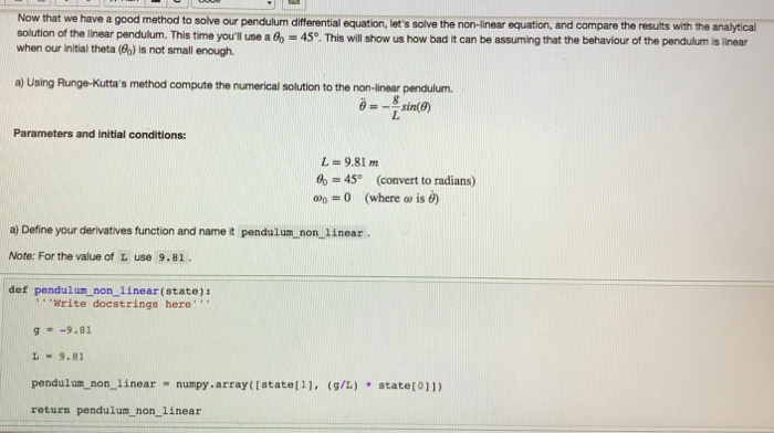
Question: Now that we have a good method to solve our pendulum differential equation, let's solve the non-linear equation, and compare the results with the analytical

Now that we have a good method to solve our pendulum differential equation, let's solve the non-linear equation, and compare the results with the analytical solution of the linear pendulum. This time youi'l use a 6 - 45. This will show us how bad t can be assuming that the behaviour of the pendulum is linear when our initial theta (0o) is not small enough. a) Using Runge-Kutta's method compute the numerical solution to the non-linear pendulunm. Parameters and initial conditions: 9.81 m ,-45 (convert to radians) 00-0 (where is a) Define your derivatives function and name it pendulum non 1inear Note: For the value of L use 9.81 def pendulum non linear (state): Write docstrings here g =-9.81 L 9.81 pendulum-non-linear -numpy . array([state[1], return pendulum non linear (g/L) state(0)))
Step by Step Solution
There are 3 Steps involved in it

Get step-by-step solutions from verified subject matter experts


