ode1 code:

% The solver implements the forward Euler method of order 1. % % Example % tspan = 0:0.1:20; % y = ode1(@vdp1,tspan,[2 0]); % plot(tspan,y(:,1)); % solves the system y' = vdp1(t,y) with a constant step size of 0.1, % and plots the first component of the solution. %

if ~isnumeric(tspan) error('TSPAN should be a vector of integration steps.'); end

if ~isnumeric(y0) error('Y0 should be a vector of initial conditions.'); end

h = diff(tspan); if any(sign(h(1))*h

try f0 = feval(odefun,tspan(1),y0,varargin{:}); catch msg = ['Unable to evaluate the ODEFUN at t0,y0. ',lasterr]; error(msg); end

y0 = y0(:); % Make a column vector. if ~isequal(size(y0),size(f0)) error('Inconsistent sizes of Y0 and f(t0,y0).'); end

neq = length(y0); N = length(tspan); Y = zeros(neq,N);

Y(:,1) = y0; for i = 1:N-1 Y(:,i+1) = Y(:,i) + h(i)*feval(odefun,tspan(i),Y(:,i),varargin{:}); end Y = Y.';

ode4 code:

function Y = ode4(odefun,tspan,y0,varargin) %ODE4 Solve differential equations with a non-adaptive method of order 4. % Y = ODE4(ODEFUN,TSPAN,Y0) with TSPAN = [T1, T2, T3, ... TN] integrates % the system of differential equations y' = f(t,y) by stepping from T0 to % T1 to TN. Function ODEFUN(T,Y) must return f(t,y) in a column vector. % The vector Y0 is the initial conditions at T0. Each row in the solution % array Y corresponds to a time specified in TSPAN. % % Y = ODE4(ODEFUN,TSPAN,Y0,P1,P2...) passes the additional parameters % P1,P2... to the derivative function as ODEFUN(T,Y,P1,P2...). % % This is a non-adaptive solver. The step sequence is determined by TSPAN % but the derivative function ODEFUN is evaluated multiple times per step. % The solver implements the classical Runge-Kutta method of order 4. % % Example % tspan = 0:0.1:20; % y = ode4(@vdp1,tspan,[2 0]); % plot(tspan,y(:,1)); % solves the system y' = vdp1(t,y) with a constant step size of 0.1, % and plots the first component of the solution. %

if ~isnumeric(tspan) error('TSPAN should be a vector of integration steps.'); end

if ~isnumeric(y0) error('Y0 should be a vector of initial conditions.'); end

h = diff(tspan); if any(sign(h(1))*h

try f0 = feval(odefun,tspan(1),y0,varargin{:}); catch msg = ['Unable to evaluate the ODEFUN at t0,y0. ',lasterr]; error(msg); end

y0 = y0(:); % Make a column vector. if ~isequal(size(y0),size(f0)) error('Inconsistent sizes of Y0 and f(t0,y0).'); end

neq = length(y0); N = length(tspan); Y = zeros(neq,N); F = zeros(neq,4);

Y(:,1) = y0; for i = 2:N ti = tspan(i-1); hi = h(i-1); yi = Y(:,i-1); F(:,1) = feval(odefun,ti,yi,varargin{:}); F(:,2) = feval(odefun,ti+0.5*hi,yi+0.5*hi*F(:,1),varargin{:}); F(:,3) = feval(odefun,ti+0.5*hi,yi+0.5*hi*F(:,2),varargin{:}); F(:,4) = feval(odefun,tspan(i),yi+hi*F(:,3),varargin{:}); Y(:,i) = yi + (hi/6)*(F(:,1) + 2*F(:,2) + 2*F(:,3) + F(:,4)); end Y = Y.';

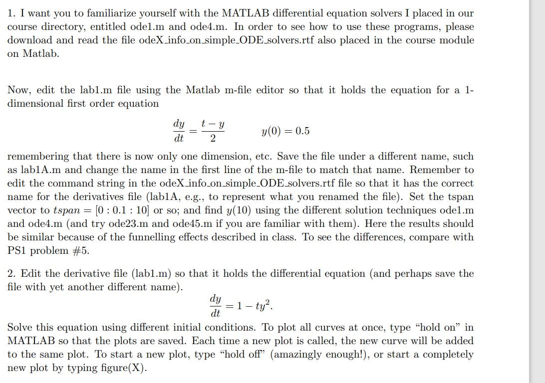
1. I want you to familiarize yourself with the MATLAB differential equation solvers I placed in our course directory, entitled ode1.m and ode4.m. In order to see how to use these programs, please download and read the file odeX_info_on_simple_ODE_solvers.rtf also placed in the course module on Matlab. Now, edit the lab1.m file using the Matlab m-file editor so that it holds the equation for a 1dimensional first order equation dtdy=2tyy(0)=0.5 remembering that there is now only one dimension, etc. Save the file under a different name, such as lab1A.m and change the name in the first line of the m-file to match that name. Remember to edit the command string in the odeX_info_on_simple_ODE_solvers.rtf file so that it has the correct name for the derivatives file (lab1A, e.g., to represent what you renamed the file). Set the tspan vector to tspan =[0:0.1:10] or so; and find y(10) using the different solution techniques ode1.m and ode4.m (and try ode23.m and ode45.m if you are familiar with them). Here the results should be similar because of the funnelling effects described in class. To see the differences, compare with PS1 problem \#5. 2. Edit the derivative file (lab1.m) so that it holds the differential equation (and perhaps save the file with yet another different name). dtdy=1ty2. Solve this equation using different initial conditions. To plot all curves at once, type "hold on" in MATLAB so that the plots are saved. Each time a new plot is called, the new curve will be added to the same plot. To start a new plot, type "hold off" (amazingly enough!), or start a completely new plot by typing figure (X)