ODE's using SIMULINK AND MATLAB

Demonstrate Example M3.1

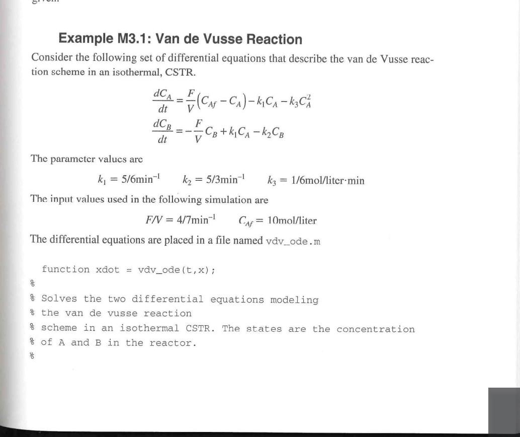
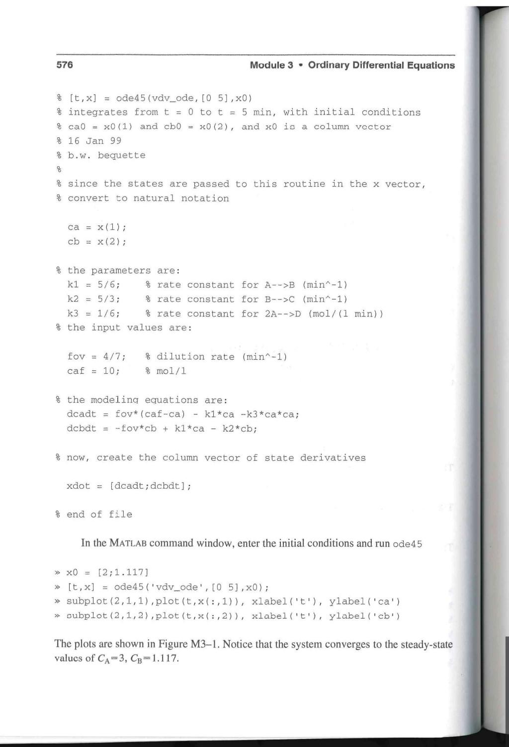
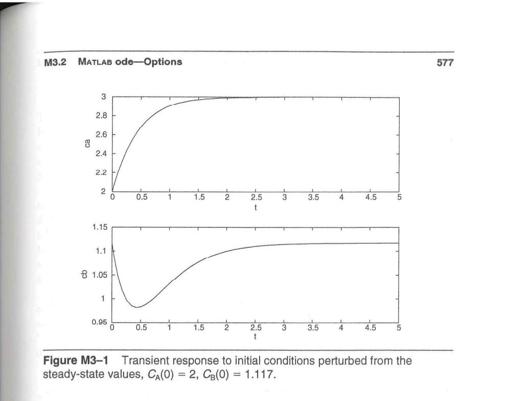
Example M3.1: Van de Vusse Reaction Consider the following set of differential equations that describe the van de Vusse reac- tion scheme in an isothermal, CSTR. dCA = 1 (CN Car -Ca)-kCA kzCk i Cg+kCA k2CB F dt V F -- dt The parameter valucs are ki = 5/6min-1 k2 = 5/3min kz = 1/6mol/liter min The input values used in the following simulation are F/V = 4/7min-1 CAF = 10mol/liter The differential equations are placed in a file named vdv_ode.m function xdot = vdv_ode (t, x); % % Solves the two differential equations modeling % the van de vusse reaction % scheme in an isothermal CSTR. The states are the concentration % of A and B in the reactor. 576 Module 3. Ordinary Differential Equations % [t,x] = ode45 (vdv_ode, [O 51, x0) % integrates from t = 0 to t = 5 min, with initial conditions % cao = x0 (1) and cb = x0(2), and xo is a column vector % 16 Jan 99 % b.w. bequette % % since the states are passed to this routine in the x vector, % convert to natural notation ca = x(1); cb = x(2); % the parameters are: k1 = 5/6; % rate constant for A-->B (min-1) k2 = 5/3; % rate constant for B-->C (min-1) k3 = 1/6; % rate constant for 2A-->D (mol/(1 min)) % the input values are: fov = 4/7; caf = 10; % dilution rate (min-1) % mol/l % the modeling equations are: dcadt = foy* (caf-ca) - k1*ca - k3*ca*ca; dcbdt = -fovicb + k1*ca - k2*cb; % now, create the column vector of state derivatives xdot = [dcadt; dcbdt]; % end of file In the MATLAB command window, enter the initial conditions and run ode45 >> X0 = [2;1.117] [t,x] = ode45 ('vdv_ode', [05], 0); subplot (2,1,1), plot(t,x(:,1)), xlabel('t'), ylabel('ca') subplot (2,1,2),plot(t, x(:,2)), xlabel('t'), ylabel('cb') The plots are shown in Figure M3-1. Notice that the system converges to the steady-state values of CA=3, CB=1.117. M3.2 MATLAB ode-Options 577 3 2.8 2.6 ca 2.4 2.2 2 0.5 1 1.5 2 3 3.5 4 4.5 5 2.5 t 1.15 1.1 8 1.05 1 0.95 0 0.5 1.5 2 3 3.5 4 4.5 5 2.5 t Figure M3-1 Transient response to initial conditions perturbed from the steady-state values, Ca(O) = 2, CB(O) = 1.117