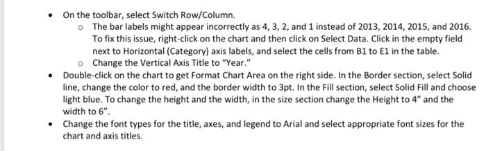
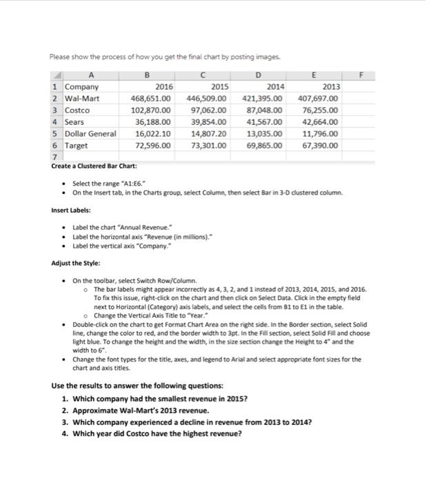
. On the toolbar, select Switch Row/Column. o The bar labels might appear incorrectly as 4, 3, 2, and 1 instead of 2013, 2014, 2015, and 2016. To fix this issue, right-click on the chart and then click on Select Data. Click in the empty field next to Horizontal (Category) axis labels, and select the cells from B1 to E1 in the table. Change the Vertical Axis Title to "Year." Double-click on the chart to get Format Chart Area on the right side. In the Border section, select Solid line, change the color to red, and the border width to 3pt. In the Fill section, select Solid Fill and choose light blue. To change the height and the width, in the size section change the Height to 4" and the width to 6". Change the font types for the title, axes, and legend to Arial and select appropriate font sizes for the chart and axis titles. Please show the process of how you get the final chart by posting images. B D E 1 Company 2015 2016 468,651.00 2014 421,395.00 2013 407,697.00 2 Wal-Mart 446,509.00 3 Costco 102,870.00 97,062.00 87,048.00 76,255.00 4 Sears 36,188.00 39,854.00 41,567.00 42,664.00 5 Dollar General 16,022.10 14,807.20 13,035.00 11,796.00 6 Target 72,596.00 73,301.00 69,865.00 67,390.00 7 Create a Clustered Bar Chart: Select the range "A1:56." On the Insert tab, in the Charts group, select Column, then select Bar in 3-D clustered column. Insert Labels: Label the chart "Annual Revenue." Label the horizontal axis "Revenue (in millions)." Label the vertical axis "Company." Adjust the Style: On the toolbar, select Switch Row/Column. The bar labels might appear incorrectly as 4, 3, 2, and 1 instead of 2013, 2014, 2015, and 2016. To fix this issue, right-click on the chart and then click on Select Data. Click in the empty field next to Horizontal (Category) axis labels, and select the cells from B1 to E1 in the table. o Change the Vertical Axis Title to "Year." Double-click on the chart to get Format Chart Area on the right side. In the Border section, select Solid line, change the color to red, and the border width to 3pt. In the Fill section, select Solid Fill and choose light blue. To change the height and the width, in the size section change the Height to 4" and the width to 6". Change the font types for the title, axes, and legend to Arial and select appropriate font sizes for the chart and axis titles. Use the results to answer the following questions: 1. Which company had the smallest revenue in 2015? 2. Approximate Wal-Mart's 2013 revenue. 3. Which company experienced a decline in revenue from 2013 to 2014? 4. Which year did Costco have the highest revenue? . On the toolbar, select Switch Row/Column. o The bar labels might appear incorrectly as 4, 3, 2, and 1 instead of 2013, 2014, 2015, and 2016. To fix this issue, right-click on the chart and then click on Select Data. Click in the empty field next to Horizontal (Category) axis labels, and select the cells from B1 to E1 in the table. Change the Vertical Axis Title to "Year." Double-click on the chart to get Format Chart Area on the right side. In the Border section, select Solid line, change the color to red, and the border width to 3pt. In the Fill section, select Solid Fill and choose light blue. To change the height and the width, in the size section change the Height to 4" and the width to 6". Change the font types for the title, axes, and legend to Arial and select appropriate font sizes for the chart and axis titles. Please show the process of how you get the final chart by posting images. B D E 1 Company 2015 2016 468,651.00 2014 421,395.00 2013 407,697.00 2 Wal-Mart 446,509.00 3 Costco 102,870.00 97,062.00 87,048.00 76,255.00 4 Sears 36,188.00 39,854.00 41,567.00 42,664.00 5 Dollar General 16,022.10 14,807.20 13,035.00 11,796.00 6 Target 72,596.00 73,301.00 69,865.00 67,390.00 7 Create a Clustered Bar Chart: Select the range "A1:56." On the Insert tab, in the Charts group, select Column, then select Bar in 3-D clustered column. Insert Labels: Label the chart "Annual Revenue." Label the horizontal axis "Revenue (in millions)." Label the vertical axis "Company." Adjust the Style: On the toolbar, select Switch Row/Column. The bar labels might appear incorrectly as 4, 3, 2, and 1 instead of 2013, 2014, 2015, and 2016. To fix this issue, right-click on the chart and then click on Select Data. Click in the empty field next to Horizontal (Category) axis labels, and select the cells from B1 to E1 in the table. o Change the Vertical Axis Title to "Year." Double-click on the chart to get Format Chart Area on the right side. In the Border section, select Solid line, change the color to red, and the border width to 3pt. In the Fill section, select Solid Fill and choose light blue. To change the height and the width, in the size section change the Height to 4" and the width to 6". Change the font types for the title, axes, and legend to Arial and select appropriate font sizes for the chart and axis titles. Use the results to answer the following questions: 1. Which company had the smallest revenue in 2015? 2. Approximate Wal-Mart's 2013 revenue. 3. Which company experienced a decline in revenue from 2013 to 2014? 4. Which year did Costco have the highest revenue