ONLY NEED CONCLUSIONS

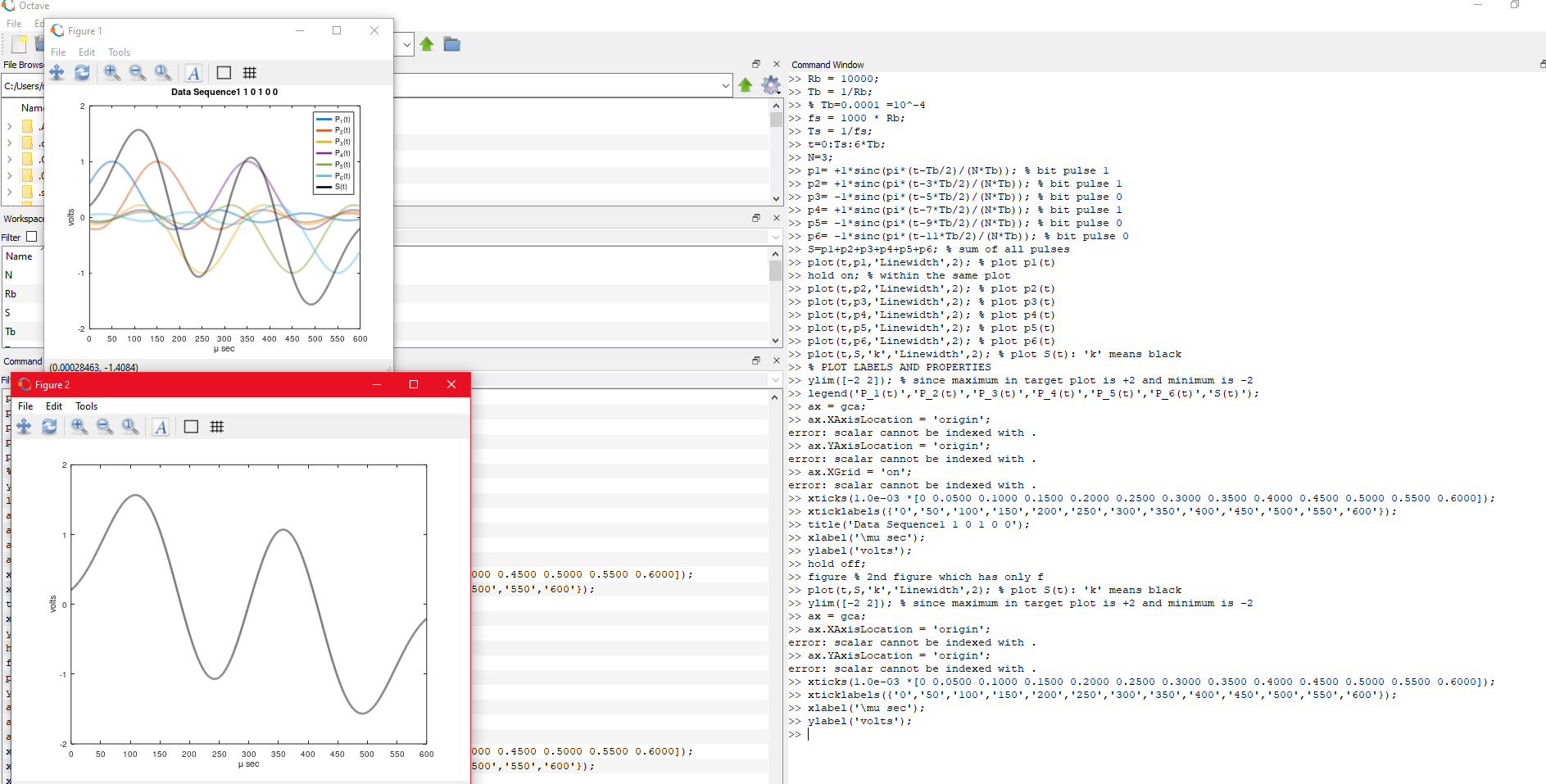
>> Rb = 10000; >> Tb = 1/Rb; >> % Tb=0.0001 =10^-4 >> fs = 1000 * Rb; >> Ts = 1/fs; >> t=0:Ts:6*Tb; >> N=3; >> p1= +1*sinc(pi*(t-Tb/2)/(N*Tb)); % bit pulse 1 >> p2= +1*sinc(pi*(t-3*Tb/2)/(N*Tb)); % bit pulse 1 >> p3= -1*sinc(pi*(t-5*Tb/2)/(N*Tb)); % bit pulse 0 >> p4= +1*sinc(pi*(t-7*Tb/2)/(N*Tb)); % bit pulse 1 >> p5= -1*sinc(pi*(t-9*Tb/2)/(N*Tb)); % bit pulse 0 >> p6= -1*sinc(pi*(t-11*Tb/2)/(N*Tb)); % bit pulse 0 >> S=p1+p2+p3+p4+p5+p6; % sum of all pulses >> plot(t,p1,'Linewidth',2); % plot p1(t) >> hold on; % within the same plot >> plot(t,p2,'Linewidth',2); % plot p2(t) >> plot(t,p3,'Linewidth',2); % plot p3(t) >> plot(t,p4,'Linewidth',2); % plot p4(t) >> plot(t,p5,'Linewidth',2); % plot p5(t) >> plot(t,p6,'Linewidth',2); % plot p6(t) >> plot(t,S,'k','Linewidth',2); % plot S(t): 'k' means black >> % PLOT LABELS AND PROPERTIES >> ylim([-2 2]); % since maximum in target plot is +2 and minimum is -2 >> legend('P_1(t)','P_2(t)','P_3(t)','P_4(t)','P_5(t)','P_6(t)','S(t)'); >> ax = gca; >> ax.XAxisLocation = 'origin'; error: scalar cannot be indexed with . >> ax.YAxisLocation = 'origin'; error: scalar cannot be indexed with . >> ax.XGrid = 'on'; error: scalar cannot be indexed with . >> xticks(1.0e-03 *[0 0.0500 0.1000 0.1500 0.2000 0.2500 0.3000 0.3500 0.4000 0.4500 0.5000 0.5500 0.6000]); >> xticklabels({'0','50','100','150','200','250','300','350','400','450','500','550','600'}); >> title('Data Sequence1 1 0 1 0 0'); >> xlabel('\mu sec'); >> ylabel('volts'); >> hold off; >> figure % 2nd figure which has only f >> plot(t,S,'k','Linewidth',2); % plot S(t): 'k' means black >> ylim([-2 2]); % since maximum in target plot is +2 and minimum is -2 >> ax = gca; >> ax.XAxisLocation = 'origin'; error: scalar cannot be indexed with . >> ax.YAxisLocation = 'origin'; error: scalar cannot be indexed with . >> xticks(1.0e-03 *[0 0.0500 0.1000 0.1500 0.2000 0.2500 0.3000 0.3500 0.4000 0.4500 0.5000 0.5500 0.6000]); >> xticklabels({'0','50','100','150','200','250','300','350','400','450','500','550','600'}); >> xlabel('\mu sec'); >> ylabel('volts'); >>

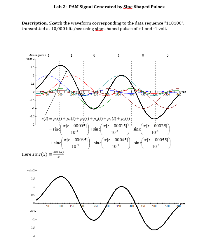
Lab 2: PAM Signal Generated by Sins-Shaped Pulses Description: Sketch the waveform corresponding to the data sequence 110100", transmitted at 10,000 bits/sec using sinc-shaped pulses of +1 and -1 volt. 1 0 1 0 0 data sequence 1 volts 2 1.5+ 1+ 0.5+ 0-13 Hec 50 100 -0.5- -1+ -1.5+ 10-4 s(t) = p.(t) + p,(t) +p:(t) +p (t) + P3 (0) + po(t) [t-00005] A[t-.00015] = sind + sind [t-00025] - sind 104 10+ t[t-00035] + sind - sind A[t-00045) - sind A[t-.00055] 10+ 10+ 104 sin (se) Here sinc(x) = volts 2 15+ 1 0.5+ OHHHHHH 50 100 150 200 250 350 400 HHH 500 450 Husec 550 640 -0.5 -1 -13+ -2 o Octave File Ed Figure 1 File Edit Tools File Brows 6 X C:/Users # Data Sequence1 10100 Nam 2 P (t) P (t) P, (t) P (t) Ps(t) P&(t) S(t) 1 > Workspac Filter o Name N Rb Tinewidth, 2): s Tb 0 50 100 150 200 250 300 350 400 450 500 550 600 u sec Command (0.00028463, -1.4084) Fil Figure 2 Command Window >> Rb = 10000; >> Tb = 1/Rb; >> Tb=0.0001 =10^-4 >> fs = 1000 * Rb; >> Ts = 1/fs; >> t=0:TS:6*Tb; >> N=3: > NES; >> pl= +1*sinc(pi* (t-Tb/2)/(N*Tb)); bit pulse 1 >> p2= +1*sinc(pi* (t-3*Tb/2)/(N*Tb)); $bit pulse i >> p3= -1*sinc (pi* (t-5*Tb/2)/(N*Tb)); } bit pulse o >> p4= +1*sinc (pi*(t-7*Tb/21/(N*Tb)); } bit pulse 1 >> p5= -1*sinc(pi* (t-9*Tb/2)/(N*Tb)); $bit pulse 0 >> p6= -1*sinc (pi* (t-11*Tb/2)/(N*Tb)); } bit pulse o >> SP-T32+23+04+5+6; sum of all pulses 3 >> plot it,pi, 'Linewidth', 2); plot pl(t) >> hold on; within the same plot >> plot(t, p2, 'Linewidth', 2); plot p2 (t) >> plot(t,p3,' plot p3 (t) >> plot(t,p4, 'Linewidth: 2); plot p4it) >> plot(t,p5, Tinewidth', 2): 3 plot p5(t) >> plot(t,p6, 'Linewidth', 2); $plot p6(t) >> plot(t, 5, 'k', 'Linewidth',2); $ plot s(t): 'k' means black >> PLOT LABELS AND PROPERTIES >> ylim( [-2 2]); $since maximum in target plot is +2 and minimum is -2 legend ('P_1(t)', 'P_2(t)','P_3(t)', 'P_4(t)', 'P_5(t)', 'P_6(t)', 'S(t)'); gca; . >> ax.XAxis Location = 'origin'; error: scalar cannot be indexed with . >> ax. YAxisLocation = 'origin'; error: scalar cannot be indexed with . >> ax. XGrid 'on'; error: scalar cannot be indexed with . >> xticks (1.0e-03 *[0 0.0500 0.1000 0.1500 0.2000 0.2500 0.3000 0.3500 0.4000 0.4500 0.5000 0.5500 0.6000]); >> xticklabels({'0', '50', '100', '150', '200', '250', '300', '350', '400', '450', '500', '550', '600'}); >> title('Data Sequencel 1010 0'); >> xlabel('\mu sec'); >> ylabel('volts'); >> hold off; >> figure $ 2nd figure which has only f >> plot(t,S,'k', 'Linewidth', 2); plot s(t): 'k' means black >> ylim( [-2 2]); $since maximum in target plot is +2 and minimum is -2 >> ax = gca; >> ax.xAxislocation = 'origin'; error: scalar cannot be indexed with . >> ax. YAxislocation = 'origin'; error: scalar cannot be indexed with . >> xticks (1.0e-03 *[0 0.0500 0.1000 0.1500 0.2000 0.2500 0.3000 0.3500 0.4000 0.4500 0.5000 0.5500 0.6000]); >> xticklabels({'0', '50', '100', '150', '200', '250', '300', '350', '400', '450', '500', '550', '600'}); >> xlabel('\mu sec'); >> ylabel('volts'); File Edit Tools - M >> ax 2 000 0.4500 0.5000 0.5500 0.6000]); 500', '550', '600' }); N 0 50 100 150 200 250 350 300 sec 400 450 500 550 600 000 0.4500 0.5000 0.5500 0.6000]); 500', '550', '600'))