Only use Matlab

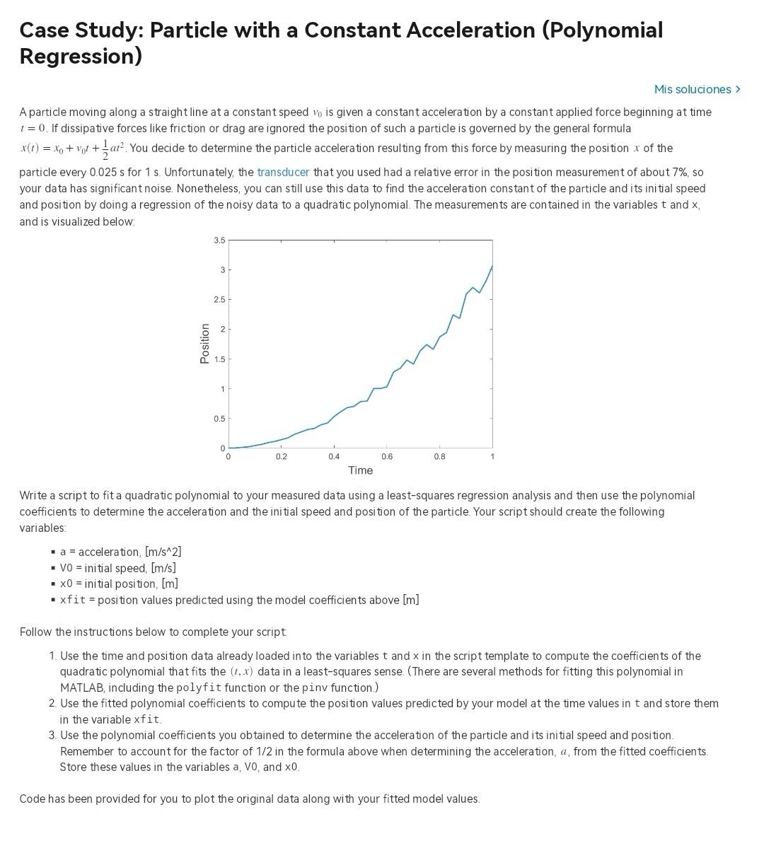
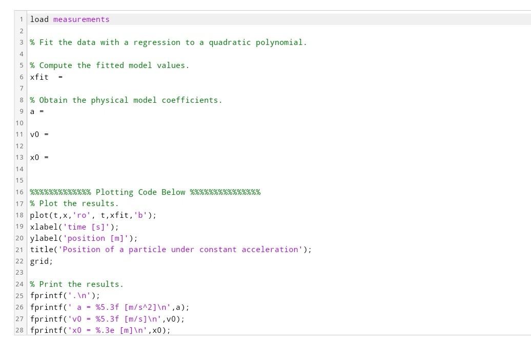
Case Study: Particle with a Constant Acceleration (Polynomial Regression) Mis soluciones A particle moving along a straight line at a constant speed v0 is given a constant acceleration by a constant applied force beginning at time t=0. If dissipative forces like friction or drag are ignored the position of such a particle is governed by the general formula x(t)=x0+v0t+21at2. You decide to determine the particle acceleration resulting from this force by measuring the position x of the particle every 0.025s for 1s. Unfortunately, the transducer that you used had a relative error in the position measurement of about 7%, so your data has significant noise. Nonetheless, you can still use this data to find the acceleration constant of the particle and its initial speed and position by doing a regression of the noisy data to a quadratic polynomial. The measurements are contained in the variables t and x, and is visualized below. Write a script to fit a quadratic polynomial to your measured data using a least-squares regression analysis and then use the polynomial coefficients to determine the acceleration and the initial speed and position of the particle. Your script should create the following variables: - a= acceleration, [m/s2] - V0 = initial speed, [m/s] - x0= initial position, [m] - xf it = position values predicted using the model coefficients above [m] Follow the instructions below to complete your script 1. Use the time and position data already loaded into the variables t and x in the script template to compute the coefficients of the quadratic polynomial that fits the (t,x) data in a least-squares sense. (There are several methods for fitting this polynomial in MATLAB, including the polyfit function or the pinv function.) 2. Use the fitted polynomial coefficients to compute the position values predicted by your model at the time values in t and store them in the variable xfit. 3. Use the polynomial coefficients you obtained to determine the acceleration of the particle and its initial speed and position. Remember to account for the factor of 1/2 in the formula above when determining the acceleration, a, from the fitted coefficients. Store these values in the variables a, Vo, and 0 Code has been provided for you to plot the original data along with your fitted model values. \% Fit the data with a regression to a quadratic polynomial. \% Compute the fitted model values. xfit = \% Obtain the physical model coefficients. a= v0= 0= %%%%%%%%%%% Plotting Code Below \%\%\%\%\%\%\%\%\%\%\%\%\% \% Plot the results. plot(t,x,ro,t,xfit,b); x label('time [s]'); ylabel ('position [m]'); title('Position of a particle under constant acceleration'); grid; \% Print the results. fprintf('. ') ; fprintf(' a=%5.3f[m/s2] ,a); fprintf(' 0=%5.3f[m/s] ,v0); fprintf (0=%.3e[m] ,x0)