Parallel computing

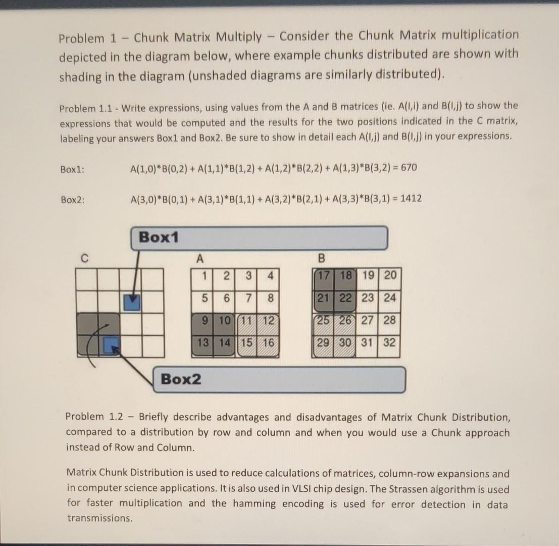
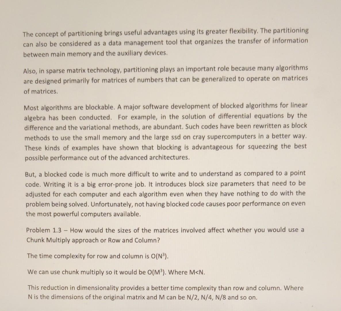
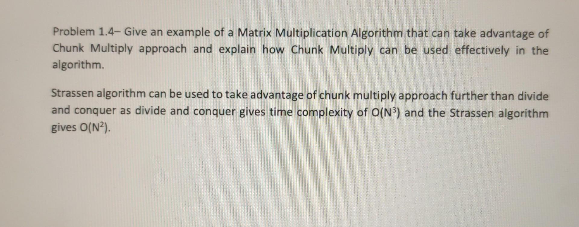
Problem 1 - Chunk Matrix Multiply - Consider the Chunk Matrix multiplication depicted in the diagram below, where example chunks distributed are shown with shading in the diagram (unshaded diagrams are similarly distributed). Problem 1.1 - Write expressions, using values from the A and B matrices (ie. A(1,i) and B(1,j) to show the expressions that would be computed and the results for the two positions indicated in the C matrix, labeling your answers Box1 and Box2. Be sure to show in detail each A(1,j) and B(1,j) in your expressions. Box1: Box2: A(1,0)B(0,2)+A(1,1)B(1,2)+A(1,2)B(2,2)+A(1,3)B(3,2)=670A(3,0)B(0,1)+A(3,1)B(1,1)+A(3,2)B(2,1)+A(3,3)B(3,1)=1412 Problem 1.2 - Briefly describe advantages and disadvantages of Matrix Chunk Distribution, compared to a distribution by row and column and when you would use a Chunk approach instead of Row and Column. Matrix Chunk Distribution is used to reduce calculations of matrices, column-row expansions and in computer science applications. It is also used in VLSI chip design. The Strassen algorithm is used for faster multiplication and the hamming encoding is used for error detection in data transmissions. The concept of partitioning brings useful advantages using its greater flexibility. The partitioning can also be considered as a data management tool that organizes the transfer of information between main memory and the auxiliary devices. Also, in sparse matrix technology, partitioning plays an important role because many algorithms are designed primarily for matrices of numbers that can be generalized to operate on matrices of matrices. Most algorithms are blockable. A major software development of blocked algorithms for linear algebra has been conducted. For example, in the solution of differential equations by the difference and the variational methods, are abundant. Such codes have been rewritten as block methods to use the small memory and the large ssd on cray supercomputers in a better way. These kinds of examples have shown that blocking is advantageous for squeezing the best possible performance out of the advanced architectures. But, a blocked code is much more difficult to write and to understand as compared to a point code. Writing it is a big error-prone job. It introduces block size parameters that need to be adjusted for each computer and each algorithm even when they have nothing to do with the problem being solved. Unfortunately, not having blocked code causes poor performance on even the most powerful computers available. Problem 1.3 - How would the sizes of the matrices involved affect whether you would use a Chunk Multiply approach or Row and Column? The time complexity for row and column is O(N3). We can use chunk multiply so it would be O(M3). Where M profile.txt % gprof -1./exeFile gmon.out > profile_line.txt % gprof -A ./exefile gmon.out > profile_anotated.txt In the flat profile we can identify the most expensive parts of the code (in this case, the calls to matsqrt, matcube, and syscube). Below are the steps taken to profile: - Call the graph profile - Visual call graph using syssqrt, matsqrt, vecsqrt, etc. Steps followed to grof: [root@thakkah] gprof - I trap.c > gprof.out [root@thakkah] more gprof.out Each sample counts as 0.01 seconds. % cumulative self self total time seconds seconds calls Ts/call Ts/call name 94.3918 .0618 .06 main (matmul_par.c:68 @ 400aea) 5.7219.151.09 main (matmul_par.c:66 @ 400b22) 0.0519 .160 .01 main (matmul_par.c:50 @ 4009f8) 0.0519 .170 .01 main (matmul_par.c:54 @ 400a57) 0.0519 .180 .01 main (matmul_par.c:70 @ 400b30) 0.0519 .190 .01 main (matmul_par.c:85 @400c39) Problem 3.2 - Use MPE for performance analysis for the implementation shown in the figure Briefly describe how the MPE output helps in your performance analysis. Note: You are expected to use Gprof with the given code in this problem and show the outputs. When using MPE, you can use instead of the long commandline a wrapper-script called mpecc/mpef77, e.g. mpecc-mpilog -o test.mpe test.c - Run the application as usually mpirun np2./trap.mpe - After the run, there is file called trap.mpe.clog 2 in the same directory - The viewer (jumpshot) unfortunately needs a different file format, so you have to convert it with clog2TOslog2 trap.mpe.clog 2 - This generates a file called trap.mpe.slog2 - You can load an slog2 file into jumpshot The viewer (jumpshot) unfortunately needs a different file format, so you have to convert it with thakkah@clog2TOslog2 trap.mpe.clog2 - This generates a file called trap.mpe.slog2 - You can load an slog2 file into jumpshot Problem 3.3 - Describe any significant performance problems in the implementation given in the figure and how you would expect any problems that you find to affect performance. Most of the code uses serialized code to calculate each process's local integral and it is also used in the integrals calculated by each process. This can be easily parallelized into MPI code using the MPI_Reduce function. Problem 3.4 - Implement a fix for any problems that you find in the given implementation., You can make changes to the code below or just show any changes you would make in your exam solution file, being careful to show exactly what could you would modify, replace or add. /*Length of each process' interval of integration = local_n*h. */ local_a = a + my_rank*local_n*h; local_b = local_a + local_n*h; MPI_Barrier(MPI_COMM_WORLD); start = MPI_Wtime(); /* Calculate each process' local integral using local endpoints*/ local_int = Trap(local_a, local_b, local_n, h); finish = MPI_Wtime(); loc_elapsed = finish-start; MPI_Reduce(\&loc_elapsed, \&elapsed, 1, MPI_DOUBLE, MPI_MAX, 0, MPI_COMM_WORLD); /*Add up the integrals calculated by each process */ MPI_Reduce(\&local_int, \&total_int, 1, MPI_DOUBLE, MPI_SUM, 0, MPI_COMM_WORLD); \#include "mpi.h" float f(floatx) float return_val; Calculate f(x)./ / Store calculation in return_val. / return_val =xx; return return_val; \}/f/<.>