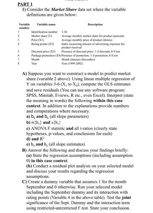
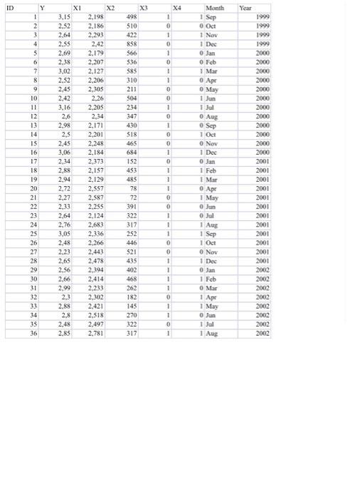
PART 1 1) Consider the Market Share data set where the variable definitions are given below: Variable Variable name Description number Identification number 1-36 Market share (Y) Average monthly market share for product (percent) Price (XI) Average monthly price of product (dolars) Rating points (X2) Index measuring amount of advertising exposure the product received Discount price (X3) Presence of discount price: l if discount, if not Package promotion (X4) Presence of promotion: 1 if promotion, if not Month Month January-December) Year Year (1999-2002) A) Suppose you want to construct a model to predict market share (variable 2 above). Using linear multiple regression of Y on variables 3-6 (X, to X), compute the OLS estimates and save residuals (You can use any software program: SPSS, Minitab, Eviews, R etc., even Excel). Interpret (state the meaning in words) the following within this case context. In addition to the explanations provide numbers and computations where necessary. a) b, and b, (all slope parameters) b) o{b} and s{b} c) ANOVA F statistic and all t-ratios (clearly state hypotheses, p-values, and conclusions for each) d) and RP e) b, and b (all slope estimates) B) Answer the following and discuss your findings briefly: (a) State the regression assumptions (including assumption 0) in this case context. (b) Conduct a residual plot analysis on your selected model and discuss your results regarding the regression assumptions. C) Create a dummy variable that assumes 1 for the month September and 0 otherwise. Run your selecetd model including the September dummy and its interaction with rating points (Variable 4 in the above table). Test the joint significance of the Sept. Dummy and the interaction term using restricted-unrestricted F test. State your conclusion. XI 3,15 2,52 2.64 2,55 2.69 X3 498 510 422 858 566 536 585 X4 Month 1 1 Sep 00 Od 1 Nov 1 Dec O Jan O Feb Mar O Ape O May 1 Jun 2.38 310 3,02 2,52 2,45 2.42 3.16 2,6 211 504 234 347 2.98 Year 1999 1999 1999 1999 2000 2000 2000 2000 2000 2000 2000 2000 2000 2000 2000 2000 2001 2001 2001 2001 2001 2001 2001 2001 2001 2,5 2,45 3,06 430 518 465 684 152 X2 2,198 2,186 2,293 2,42 2,179 2,207 2,127 2.206 2,305 2.26 2,205 2,34 2,171 2,201 2,248 2.184 2,373 2,157 2,129 2.557 2,587 2,255 2,124 2,683 2,336 2,266 2.443 2.478 2,394 2.414 2.233 2,302 2.421 2.518 2,497 2.781 dici 453 485 2,72 O Aug O Sep 1 Oct Dec 0 Jan 1 Feb 1 Mar 0 Apr 1 May Jun 1 O Jul 11 Aug 1 Sep 1 Oct O Nov 1 Dec 0 Jan 1 1 Feb O Mar 0 1 Apr 1 May 1 0 Jun 0 1 Jul 11 Aug 391 322 317 252 446 521 2,48 2001 2.23 2,56 2.66 2,99 2,3 2.88 402 468 262 182 2001 2001 2002 2002 2002 2002 2002 2002 2002 2002 145 270 2.8 2,48 2.85 322 317 36 PART 1 1) Consider the Market Share data set where the variable definitions are given below: Variable Variable name Description number Identification number 1-36 Market share (Y) Average monthly market share for product (percent) Price (XI) Average monthly price of product (dolars) Rating points (X2) Index measuring amount of advertising exposure the product received Discount price (X3) Presence of discount price: l if discount, if not Package promotion (X4) Presence of promotion: 1 if promotion, if not Month Month January-December) Year Year (1999-2002) A) Suppose you want to construct a model to predict market share (variable 2 above). Using linear multiple regression of Y on variables 3-6 (X, to X), compute the OLS estimates and save residuals (You can use any software program: SPSS, Minitab, Eviews, R etc., even Excel). Interpret (state the meaning in words) the following within this case context. In addition to the explanations provide numbers and computations where necessary. a) b, and b, (all slope parameters) b) o{b} and s{b} c) ANOVA F statistic and all t-ratios (clearly state hypotheses, p-values, and conclusions for each) d) and RP e) b, and b (all slope estimates) B) Answer the following and discuss your findings briefly: (a) State the regression assumptions (including assumption 0) in this case context. (b) Conduct a residual plot analysis on your selected model and discuss your results regarding the regression assumptions. C) Create a dummy variable that assumes 1 for the month September and 0 otherwise. Run your selecetd model including the September dummy and its interaction with rating points (Variable 4 in the above table). Test the joint significance of the Sept. Dummy and the interaction term using restricted-unrestricted F test. State your conclusion. XI 3,15 2,52 2.64 2,55 2.69 X3 498 510 422 858 566 536 585 X4 Month 1 1 Sep 00 Od 1 Nov 1 Dec O Jan O Feb Mar O Ape O May 1 Jun 2.38 310 3,02 2,52 2,45 2.42 3.16 2,6 211 504 234 347 2.98 Year 1999 1999 1999 1999 2000 2000 2000 2000 2000 2000 2000 2000 2000 2000 2000 2000 2001 2001 2001 2001 2001 2001 2001 2001 2001 2,5 2,45 3,06 430 518 465 684 152 X2 2,198 2,186 2,293 2,42 2,179 2,207 2,127 2.206 2,305 2.26 2,205 2,34 2,171 2,201 2,248 2.184 2,373 2,157 2,129 2.557 2,587 2,255 2,124 2,683 2,336 2,266 2.443 2.478 2,394 2.414 2.233 2,302 2.421 2.518 2,497 2.781 dici 453 485 2,72 O Aug O Sep 1 Oct Dec 0 Jan 1 Feb 1 Mar 0 Apr 1 May Jun 1 O Jul 11 Aug 1 Sep 1 Oct O Nov 1 Dec 0 Jan 1 1 Feb O Mar 0 1 Apr 1 May 1 0 Jun 0 1 Jul 11 Aug 391 322 317 252 446 521 2,48 2001 2.23 2,56 2.66 2,99 2,3 2.88 402 468 262 182 2001 2001 2002 2002 2002 2002 2002 2002 2002 2002 145 270 2.8 2,48 2.85 322 317 36