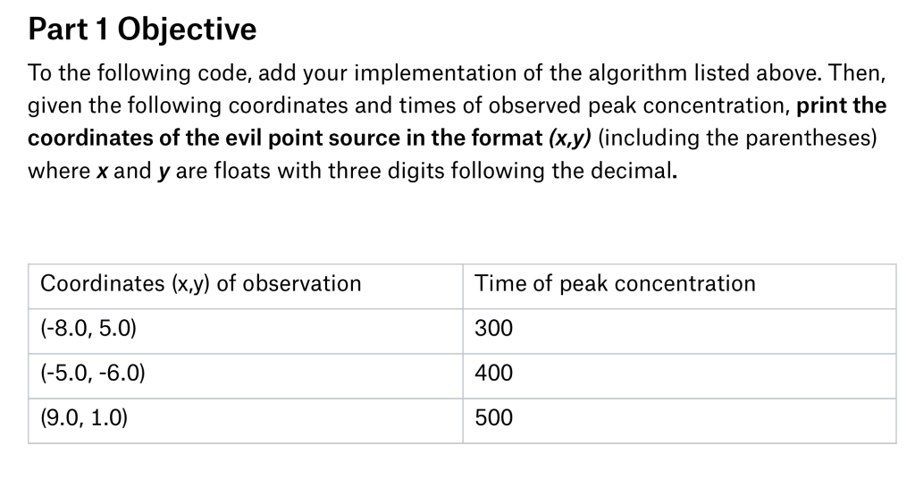
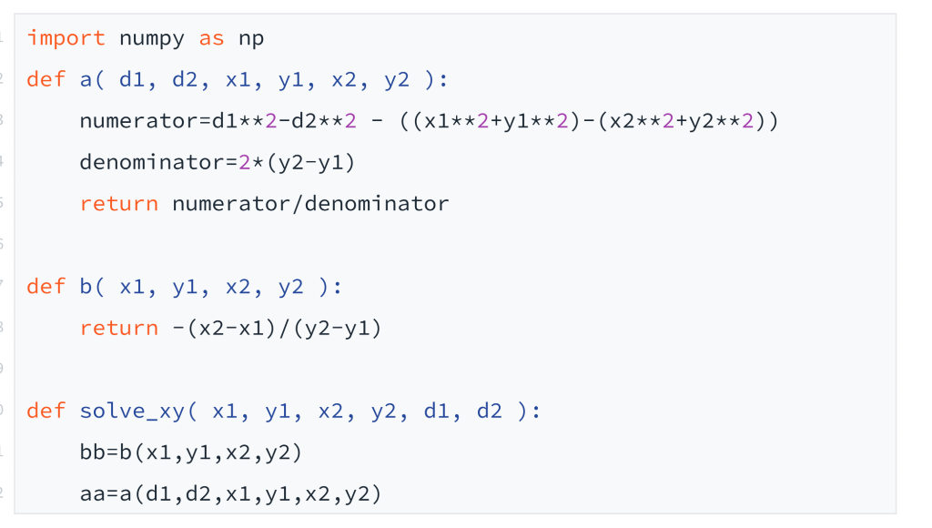
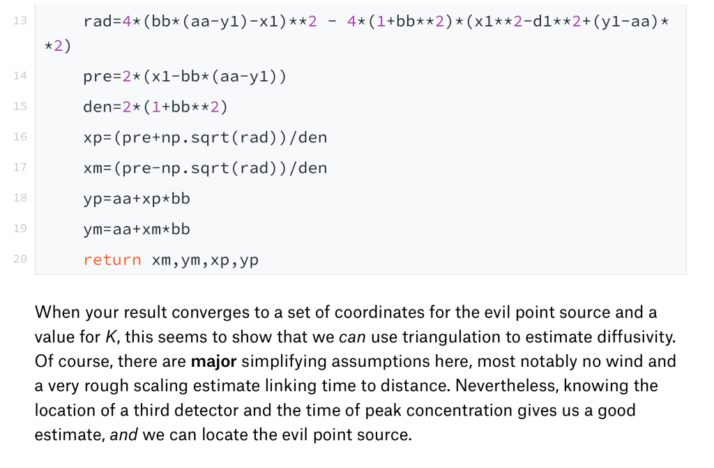
Part 1 Objective To the following code, add your implementation of the algorithm listed above. Then, given the following coordinates and times of observed peak concentration, print the coordinates of the evil point source in the format (x.y) (including the parentheses) where x and y are floats with three digits following the decimal. Coordinates (x.y) of observation (-8.0, 5.0) Time of peak concentration 300 400 500 import numpy as np def a( dl, d2, xl, yl, x2, y2 : numerator dl**2-d2**2 - ((xl**2+yl**2)-(x2**2+y2**2)) denominator-2* (y2-y1) return numerator/denominator def b( xl, yl, x2, y2): return -(x2-x1)/ (y2-yl) def solve xy( x1, yl, x2, y2, d1, d2 ): bb-b(x1,yl,x2,y2) aa-a (dl,d2,x1, yl,x2,y2) 13 pre-2* (x1-bb* (aa-yl)) den-2* (1+bb**2) xp (pre+np.sqrt (rad))/den xm- (pre-np.sqrt(rad))/den yp-aa+xpbb ym-aa+xm*bb return Xm, ym, xp,yp 14 15 16 17 18 19 When your result converges to a set of coordinates for the evil point source and a value for K, this seems to show that we can use triangulation to estimate diffusivity. Of course, there are major simplifying assumptions here, most notably no wind and a very rough scaling estimate linking time to distance. Nevertheless, knowing the location of a third detector and the time of peak concentration gives us a good estimate, and we can locate the evil point source. Part 1 Objective To the following code, add your implementation of the algorithm listed above. Then, given the following coordinates and times of observed peak concentration, print the coordinates of the evil point source in the format (x.y) (including the parentheses) where x and y are floats with three digits following the decimal. Coordinates (x.y) of observation (-8.0, 5.0) Time of peak concentration 300 400 500 import numpy as np def a( dl, d2, xl, yl, x2, y2 : numerator dl**2-d2**2 - ((xl**2+yl**2)-(x2**2+y2**2)) denominator-2* (y2-y1) return numerator/denominator def b( xl, yl, x2, y2): return -(x2-x1)/ (y2-yl) def solve xy( x1, yl, x2, y2, d1, d2 ): bb-b(x1,yl,x2,y2) aa-a (dl,d2,x1, yl,x2,y2) 13 pre-2* (x1-bb* (aa-yl)) den-2* (1+bb**2) xp (pre+np.sqrt (rad))/den xm- (pre-np.sqrt(rad))/den yp-aa+xpbb ym-aa+xm*bb return Xm, ym, xp,yp 14 15 16 17 18 19 When your result converges to a set of coordinates for the evil point source and a value for K, this seems to show that we can use triangulation to estimate diffusivity. Of course, there are major simplifying assumptions here, most notably no wind and a very rough scaling estimate linking time to distance. Nevertheless, knowing the location of a third detector and the time of peak concentration gives us a good estimate, and we can locate the evil point source