Part a) should have 12 equations total.

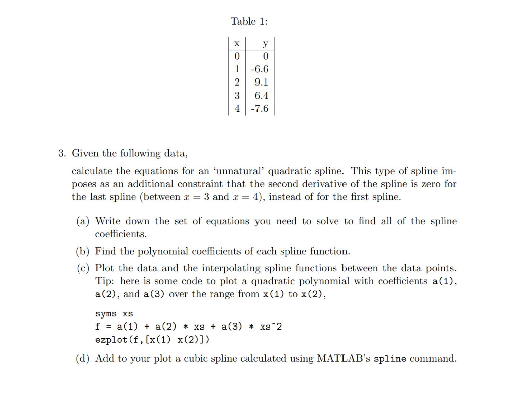
Table 1 0 1 -6.6 2 9.1 3 6.4 3. Given the following data, calculate the equations for an 'unnatural' quadratic spline. This type of spline im poses as an additional constraint that the second derivative of the spline is zero for the last spline (between 3 and 4), instead of for the first spline (a) Write down the set of equations you need to solve to find a of the spline coefficients (b) Find the polynomal coefficients of each spline function. (c) Plot the data and the interpolating spline functions between the data points Tip: here is some code to plot a quadratic polynomial with coefficients a1) a (2), and a(3) over the range from x(1) to x (2) syms xS f = a(1) + a(2) * xs + a(3) * xs*2 ezplot (f, [x(1) x(2)1) (d) Add to your plot a cubic spline calculated using MATLAB's spline command. Table 1 0 1 -6.6 2 9.1 3 6.4 3. Given the following data, calculate the equations for an 'unnatural' quadratic spline. This type of spline im poses as an additional constraint that the second derivative of the spline is zero for the last spline (between 3 and 4), instead of for the first spline (a) Write down the set of equations you need to solve to find a of the spline coefficients (b) Find the polynomal coefficients of each spline function. (c) Plot the data and the interpolating spline functions between the data points Tip: here is some code to plot a quadratic polynomial with coefficients a1) a (2), and a(3) over the range from x(1) to x (2) syms xS f = a(1) + a(2) * xs + a(3) * xs*2 ezplot (f, [x(1) x(2)1) (d) Add to your plot a cubic spline calculated using MATLAB's spline command