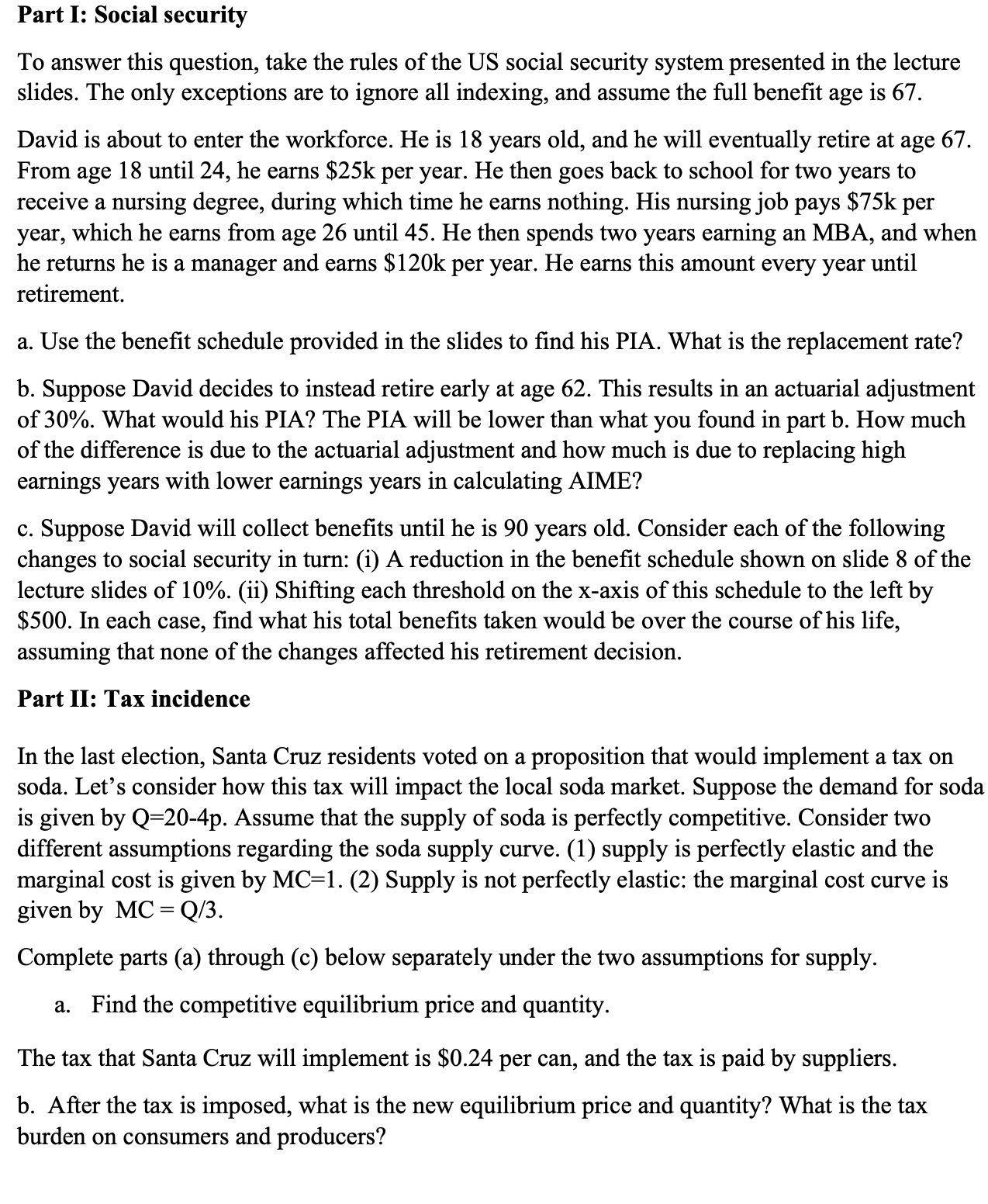
Part I: Social security

To answer this question, take the rules of the US social security system presented in the lecture slides. The only exceptions are to ignore all indexing, and assume the full benefit age is $67.$

David is about to enter the workforce. He is $18$ years old, and he will eventually retire at age $67.$ From age $18$ until $24,$ he earns $\backslash (\backslash$$ $25$ k $\backslash )$ per year. He then goes back to school for two years to receive a nursing degree, during which time he earns nothing. His nursing job pays $\backslash (\backslash$$ $75\backslash$mathrm$\{$k$\}\backslash )$ per year, which he earns from age $26$ until $45.$ He then spends two years earning an MBA, and when he returns he is a manager and earns $\backslash (\backslash$$ $120\backslash$mathrm$\{$k$\}\backslash )$ per year. He earns this amount every year until retirement.

a$.$ Use the benefit schedule provided in the slides to find his PIA. What is the replacement rate?

b$.$ Suppose David decides to instead retire early at age $62.$ This results in an actuarial adjustment of $\backslash (30\backslash \%\backslash ).$ What would his PIA? The PIA will be lower than what you found in part b$.$ How much of the difference is due to the actuarial adjustment and how much is due to replacing high earnings years with lower earnings years in calculating AIME?

c$.$ Suppose David will collect benefits until he is $90$ years old. Consider each of the following changes to social security in turn: $($i$)$ A reduction in the benefit schedule shown on slide $8$ of the lecture slides of $\backslash (10\backslash \%\backslash ).($ii$)$ Shifting each threshold on the x $-$axis of this schedule to the left by $\backslash (\backslash$$ $500\backslash ).$ In each case, find what his total benefits taken would be over the course of his life, assuming that none of the changes affected his retirement decision.

Part II: Tax incidence

In the last election, Santa Cruz residents voted on a proposition that would implement a tax on soda. Let's consider how this tax will impact the local soda market. Suppose the demand for soda is given by $\backslash (\backslash$mathrm$\{$Q$\}=20-4\backslash$mathrm$\{$p$\}\backslash ).$ Assume that the supply of soda is perfectly competitive. Consider two different assumptions regarding the soda supply curve. $(1)$ supply is perfectly elastic and the marginal cost is given by $\backslash (\backslash$mathrm$\{$MC$\}=1\backslash ).(2)$ Supply is not perfectly elastic: the marginal cost curve is given by $\backslash (\backslash$mathrm$\{$MC$\}=\backslash$mathrm$\{$Q$\}/3\backslash ).$

Complete parts $($a$)$ through $($c$)$ below separately under the two assumptions for supply.

a$.$ Find the competitive equilibrium price and quantity.

The tax that Santa Cruz will implement is $\backslash (\backslash$$ $0\mathrm{.}24\backslash )$ per can, and the tax is paid by suppliers.

b$.$ After the tax is imposed, what is the new equilibrium price and quantity? What is the tax burden on consumers and producers?

c$.$ Calculate the deadweight loss of the tax.

d$.$ How does the incidence and deadweight loss compare and why? Which assumption for supply do you think is more realistic for the Santa Cruz market?