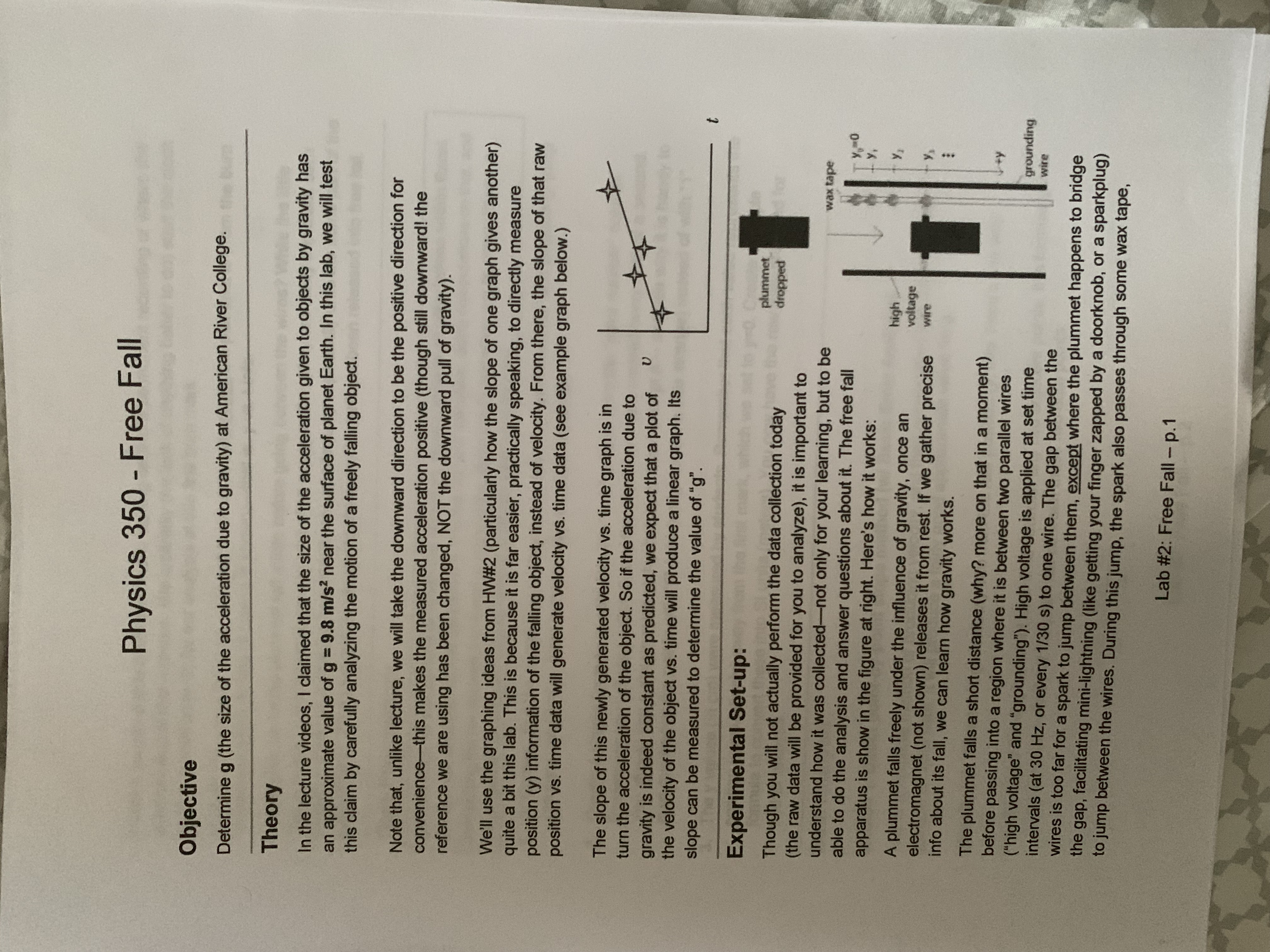
Physics 350 - Free Fall Objective Determine g (the size of the acceleration due to gravity) at American River College. Theory In the lecture videos, I claimed that the size of the acceleration given to objects by gravity has an approximate value of g = 9.8 m/s? near the surface of planet Earth. In this lab, we will test this claim by carefully analyzing the motion of a freely falling object. Note that, unlike lecture, we will take the downward direction to be the positive direction for convenience-this makes the measured acceleration positive (though still downward! the reference we are using has been changed, NOT the downward pull of gravity). We'll use the graphing ideas from HW#2 (particularly how the slope of one graph gives another) quite a bit this lab. This is because it is far easier, practically speaking, to directly measure position (y) information of the falling object, instead of velocity. From there, the slope of that raw position vs. time data will generate velocity vs. time data (see example graph below.) The slope of this newly generated velocity vs. time graph is in turn the acceleration of the object. So if the acceleration due to gravity is indeed constant as predicted, we expect that a plot of U the velocity of the object vs. time will produce a linear graph. Its slope can be measured to determine the value of "g". Experimental Set-up: plummet Though you will not actually perform the data collection today dropped (the raw data will be provided for you to analyze), it is important to understand how it was collected-not only for your learning, but to be wax tape able to do the analysis and answer questions about it. The free fall apparatus is show in the figure at right. Here's how it works: y, A plummet falls freely under the influence of gravity, once an high voltage electromagnet (not shown) releases it from rest. If we gather precise wire info about its fall, we can learn how gravity works. : The plummet falls a short distance (why? more on that in a moment) before passing into a region where it is between two parallel wires ("high voltage" and "grounding"). High voltage is applied at set time grounding intervals (at 30 Hz, or every 1/30 s) to one wire. The gap between the wire wires is too far for a spark to jump between them, except where the plummet happens to bridge the gap, facilitating mini-lightning (like getting your finger zapped by a doorknob, or a sparkplug) to jump between the wires. During this jump, the spark also passes through some wax tape, Lab #2: Free Fall - p.1where it causes a little black burn mark, leaving behind a permanent recording of where the plummet was at that moment. We arbitrarily (for lack of anything better to do) start the clock 1=0) and position (y=0) for our analysis at this first burn mark. In short, this whole fancy set-up is just to tell us exactly where the plummet is (from the burn marks) and when (timing of sparks is known)-that is, y vs. t info. And why do we let the plummet fall a little before going between the wires? While the little "flame marks" in the figure above are a bit of an exaggeration (they are really tiny black burn marks), it would be a true fire hazard to let the sparks jump repeatedly onto the same part of the tape-that is, if the plummet is not moving, because it hasn't yet been released into free fall. Data Preparation: General note: for this lab (and all others this semester), please perform all calculations within Excel, so I can see what you did and troubleshoot. (Pulling out your calculator, doing computations on that, and then putting the results back into Excel, is missing the whole point!) And when you do computations in Excel, please use adjacent cells as needed to clearly label what they are. 1. In Canvas, find the sample set of data for this lab. The "point number" and position (y [cm]) columns are filled in. Note that the "point number" starts with "0." 2. Create a simple formula to calculate the "time" column from the "point number" column. Remember you will start with t=0, and that there is a mark created every 1/30 of a second. You should see a simple relationship between "time" and "pt #"-- and see why it is handy to start numbering the points with "0" (which might seem a little strange) instead of with "1". 3. The y values (in cm) were measured by students. Remember that each value represents the position (cumulatively) away from the first mark, which we set to y=0. Create a simple formula to convert these into SI units (meters). You now have the raw data prepared for further analysis. Data Analysis: Method 1: Direct point-by-point slope method (w/ Basic Error Analysis) This is an intuitive method of producing velocity, and then acceleration info, from the raw position vs. time data. It will produce a fairly good approximate value for g. Velocity (v): We want to get velocity info from the raw position (y) info. Here's one way: If we figure out the displacement over time between any two adjacent points, this formula gives the average velocity of the plummet between those two data points: V av Ay _( ) s - yi ) At At (1) Lab #2: Free Fall - p.2If we assume that the data points are made often enough that the object doesn't have a chance to change velocity much from the beginning to the end of the time interval, then we can assume, without losing too much accuracy, Vav is similar to vi (and to be fair, vi also, though we won't have use for that): Vav = VF (= Vi) ( 2 ) This gives us a way to estimate the instantaneous velocity info at any given time point: vat time t) = [y(at time t) - y(at previous data pt) (3) At The time between adjacent points (At) is fixed at 1/30 s, per the setting of the apparatus. Acceleration (a): Using the fact that the acceleration is given by the slope of v vs. t, you can use the same logic to eqn #1-3 (as well as similar Excel work) to generate approximate acceleration info: a ( at time t) = [v(at time t) - v(at previous data pt)] ( 4 ) At 4. Program the velocity column on your spreadsheet using eqn (3). Note that you need to leave the first velocity value blank (marked [n/a))-since to calculate a value from eqn (3) requires a previous data point for "y" to refer to, which doesn't exist yet for the first row. (Do not overwrite "n/a" with 0 as that is not correct. We will explore this later; this is a limitation of Method 1, but not of Method 2 which we'll do next.) 5. Add an acceleration column to your spreadsheet using eqn (4). For the same reason, you will now need to leave the first two acceleration values blank (marked [n/a))-that is, until you have a velocity value from the previous row to refer to. 6. Take a look at your acceleration column, and you should (hopefully) notice that, while the values fluctuate, it is nonetheless around a constant value, not increasing or decreasing as a general trend. If so, you are seeing that the acceleration is constant, to within experimental error. (If the data points fluctuate a bit around a linear trend, so will the point-to-point slopes.) Take the average of your acceleration column, using Excel (see "How to Use Excel" p. 1). Then calculate (in Excel!) the % error (your value vs. the accepted theoretical value.) Also record it on the result sheet in the back of this lab (always including units.) 1 If the units of any quantity-from a graph, or otherwise- aren't already clear to you, remember to use what you learned in Lab #1 (Part 2, step 3b) to figure out what they should be. Lab #2: Free Fall - p.37. Graphing the data: Please make two graphs: of y vs. t and v vs. t in your spreadsheet. Follow along carefully with the graphing steps ("How to Use Excel" p. 3-4)-and as in lab #1, no need to do step 3 this semester and no need for steps 6-7 today (always by request only). Also remember from lab #1 how to graph columns that are non-adjacent, as necessary. Note: for the v vs. t graph, make sure to use equal length columns- select the data starting with the 2nd row (the first one where both have values.) A "I" without a "v" cannot be plotted! Method 2: Linear Least Squares Fit method We already mentioned that there were some approximations inherent in our method #1 (eqn 2 for v-and similarly for acceleration). To refine our analysis a bit, we'll now use our powerful linear fit techniques from lab #1, at least once we have a relationship (velocity vs. time) that is supposed to be linear. 8. Perform a linear fit on your v vs. t data (using Excel's linest). Show your calculations in Excel and also record on your result sheet, including units. (Do NOT accidentally do this on your y vs. t data- it is not expected to be linear!). Remember to make sure (for this and all future labs!) that your R2 value is NOT showing as "1" exactly, increasing the number of decimal places displayed as needed. (Why? See Lab #1 reference materials about R2.) 9. From this info, write down this method's most probable value of the acceleration due to gravity () and then compute the 95% confidence interval for the value of g. Include units! Show your calculations in Excel and also record them on the result sheet. Then perform the same analysis on the vertical axis intercept (b) of your graph. In the final questions below, you will be asked to interpret the physical meaning of this quantity. Final Questions: For the y vs. t graph: (Questions #1-2) 1.) Which best describes the shape of your graph? (Underline/bold your choice.) linear curved w/ slope increase curved w/ slope decrease 2.) What physical quantity does the slope of this graph represent? Is this consistent with your answer from #1? Explain.For the v vs. t graph: (Questions #3-10) 3.) a.) Which best describes the shape of your graph? (Underline/bold your choice.) linear curved w/ slope increase curved w/ slope decrease b.) How does the R2 value from your linest help you to rigorously determine this? (Hint: see "Error Analysis" document.) Slope (of v vs. t): (Questions #4-6) 4.) What physical quantity does the slope of this graph represent? Is this consistent with your answer from #3? Explain. 5.) Does the accepted value of g fall within your confidence interval from method 2? What does that tell you? 6.) What would be the most likely source of error in this experiment? (Hint: see lecture notes.) Explain if this would tend to throw off experimental values higher or lower (vs. theory). And do you see any (statistically significant) evidence of this factor in your results? Lab #2: Free Fall - p.5Vertical axis intercept (of v vs. t): (Questions #7-10) 7.) What physical quantity does the vertical intercept of this graph represent? Explain. 8.) Is your experimental value statistically distinguishable from zero? (Hint: Use your 95% C.1.) 9.) Explain, in practical terms, why the vertical axis intercept isn't zero. (Hint: think about the apparatus design.) 10.) Why is it not important (to the goals of this lab) for the vertical intercept to be zero? What to submit: In Canvas, upload: your spreadsheet (.xIsx format) all calculations done within it & two graphs (y vs. t, v vs. t) this document (pdf format preferred) with all questions above answered & results sheet filled in below Lab #2: Free Fall - p.6Results Sheet METHOD 1: Direct point-by-point slope with Basic Error Analysis Include units! g (experimental, avg) (accepted) % error METHOD 2: Linear Least Squares Fit (v vs. t) Parameter: Numerical value: Units: O O R2 n/a Experimental estimate for g: (include units!) = Ocgs = 2 0 = 0