Please answer exercises 11.4.4 and 11.4.5 Stepwise

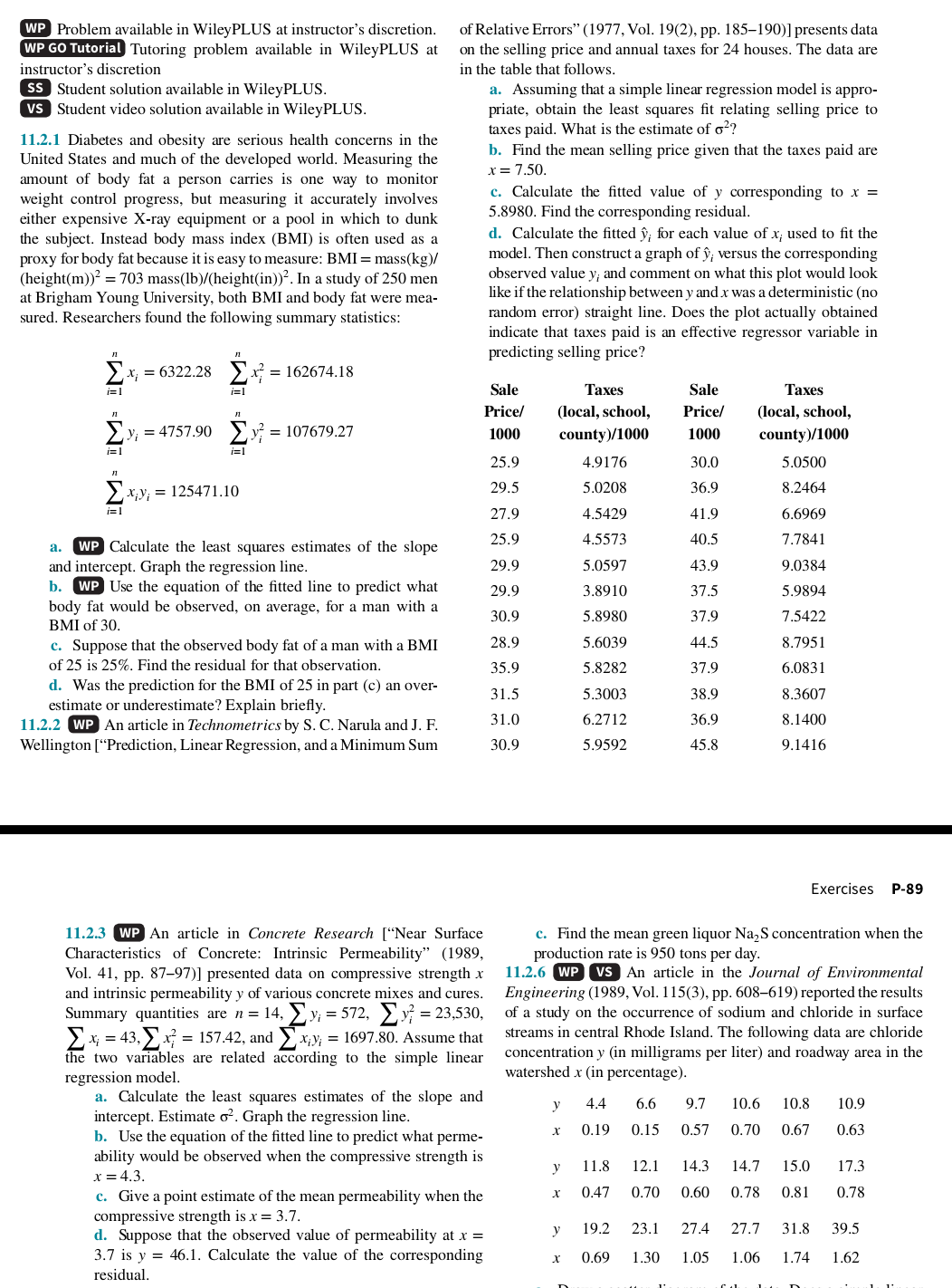
11.4.4 Consider the data from Exercise 11.2.2 on y = sales price and x = taxes paid. a. Test H,: B, = 0 using the r-test; use a = 0.05. b. Test Hy: B, = 0 using the analysis of variance with = 0.05. Discuss the relationship of this test to the test from part (a). c. Estimate the standard errors of the slope and intercept. d. Test the hypothesis that B, = 0. 11.4.5 Consider the data from Exercise 11.2.3 on x = compres- sive strength and y = intrinsic permeability of concrete. a. Test for significance of regression using a = 0.05. Find the P-value for this test. Can you conclude that the model specifies a useful linear relationship between these two variables? b. Estimate o7 and the standard deviation of B,. c. What is the standard error of the intercept in this model? cD Problem available in WileyPLUS at instructor's discretion. Tutoring problem available in WileyPLUS at instructor's discretion e& Student solution available in WileyPLUS. Student video solution available in WileyPLUS. 11.2.1 Diabetes and obesity are serious health concerns in the United States and much of the developed world. Measuring the amount of body fat a person carries is one way to monitor weight control progress, but measuring it accurately involves either expensive X-ray equipment or a pool in which to dunk the subject. Instead body mass index (BMI) is often used as a proxy for body fat because itis easy to measure: BMI = mass(kg)/ (height(m)) = 703 mass(Ib)/(height(in))*. In a study of 250 men at Brigham Young University, both BMI and body fat were mea- sured. Researchers found the following summary statistics: y x, = 6322.28 y x i=! i=! 162674.18 Sale Taxes Sale Taxes n n Price/ (local, school, Price/ (local, school, >! y, =4757.90 } y? = 107679.27 1000s county)/1000 ~=:1000-county)/1000 i=l i=l 25.9 4.9176 30.0 5.0500 > x,y, = 125471.10 29.5 3.0208 36.9 $.2464 a 27.9 4.5429 41.9 6.6969 a. cD Calculate the least squares estimates of the slope 25.9 4.5373 40.5 7.7841 and intercept. Graph the regression line. 29.9 5.0597 43.9 9.0384 b. CD Use the equation of the fitted line to predict what 39.9 3.29010 37.5 5.9894 body fat would be observed, on average, for a man with a 59 BMI of 30. 30.9 5.8980 37.9 7.5422 c. Suppose that the observed body fat of aman with a BMI 28.9 5.6039 44.5 8.7951 of 25 is 25%. Find the residual for that observation. 35.9 5.8282 37.9 6.0831 d. Was the prediction for the BMI of 25 in part (c) an over 315 53003 38.9 8 3607 estimate or underestimate? Explain briefly. 11.2.2 cD An article in Technometrics by S.C. Narula and J. F. 31.0 6.2712 36.9 8.1400 Wellington [\"Prediction, Linear Regression, and a Minimum Sum 30.9 5.9592 45.8 9.1416 Exercises 11.2.3 QJ An article in Concrete Research [Near Surface c. Find the mean green liquor Na;S concentration when the of Relative Errors\" (1977, Vol. 19(2), pp. 185-190)] presents data on the selling price and annual taxes for 24 houses. The data are in the table that follows. a. Assuming that a simple linear regression model is appro- priate, obtain the least squares fit relating selling price to taxes paid. What is the estimate of 07? b. Find the mean selling price given that the taxes paid are x= 7.50. c. Calculate the fitted value of y corresponding to x = 5.8980. Find the corresponding residual. d. Calculate the fitted }, for each value of x; used to fit the model. Then construct a graph of }, versus the corresponding observed value y; and comment on what this plot would look like if the relationship between y and x was a deterministic (no random error) straight line. Does the plot actually obtained indicate that taxes paid is an effective regressor variable in predicting selling price? Characteristics of Concrete: Intrinsic Permeability\" (1989, Vol. 41, pp. 87-97)] presented data on compressive strength x and intrinsic permeability y of various concrete mixes and cures. Summary quantities are n = 14, yy = 572, > ye = 23,530, x, = 43.) x = 157.42, and x; = 1697.80. Assume that the two variables are related according to the simple linear regression model. a. Calculate the least squares estimates of the slope and intercept. Estimate o*. Graph the regression line. b. Use the equation of the fitted line to predict what perme- ability would be observed when the compressive strength is x=4.3. c. Give a point estimate of the mean permeability when the compressive strength is x = 3.7. d. Suppose that the observed value of permeability at x = 3.7 is y = 46.1. Calculate the value of the corresponding residual. production rate is 950 tons per day. 11.2.6 cs An article in the Journal of Environmental Engineering (1989, Vol. 115(3), pp. 608-619) reported the results of a study on the occurrence of sodium and chloride in surface streams in central Rhode Island. The following data are chloride concentration y (in milligrams per liter) and roadway area in the watershed x (in percentage). y 44 6.6 97 10.6 108 10.9 x O19 O15 O57 0.70 0.67 0.63 y 118 12.1 143 14.7 15.0 17.3 x O47 0.70 0.60 0.78 0.81 0.78 y 19.2 23.1 274 27.7) 318 395 x 0.69 1.30 1.05 1.06 1.74 1.62 m aa. a" wa ros " 1 4"