please answer using excel with formulas please! thank you! I've tried looking at many other examples and they were to hard to understand so i could figure it out for myself

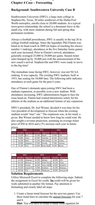
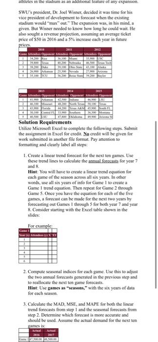
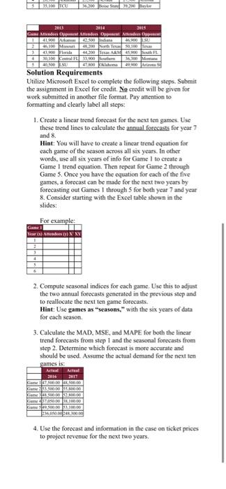
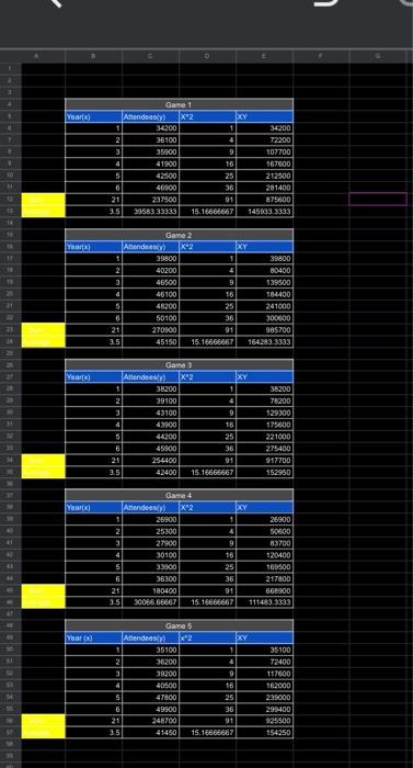
Chapter 4 Case - Forecasting Background: Southwestern University Case B Southwestern University (SWU), a large state college in Stephenville, Texas, 30 miles southwest of the Dallas/Fort Worth metroplex, enrolls close to 20,000 students. In a typical town-gown relationship, the school is a dominant force in the small city, with more students during fall and spring than permanent residents Always a football powerhouse, SWU is usually in the top 20 in college football rankings. Since the legendary Phil Flamm was hired as its head coach in 2009 (in hopes of reaching the clusive number 1 ranking), attendance at the five Saturday home games each year increased. Prior to Flamm's arrival, attendance generally averaged 25,000 to 29,000 per game. Season ticket sales bumped up by 10,000 just with the announcement of the new coach's arrival. Stephenville and SWU were ready to move to the big time! The immediate issue facing SWU, however, was not NCAA ranking. It was capacity. The existing SWU stadium, built in 1953, has seating for 54,000 fans. The following table indicates attendance at each game for the past 6 years. One of Flamm's demands upon joining SWU had been a Stadium expansion, or possibly even a new stadium. With attendance increasing, SWU administrators began to face the issue head-on. Flamm had wanted dormitories solely for his athletes in the stadium as an additional feature of any expansion SWU's president, Dr. Joel Wiszer. decided it was time for his vice president of development to forecast when the existing stadium would "max" out." The expansion was, in his mind, a given. But Wisner needed to know how long he could wait. He also sought a revenue projection, assuming an average ticket price of $50 in 2016 and a 5% increase cach year in future prices 200 3.2 Game Andres Oppones De Anders 1142300 100 M 35. SC 10.00 10,300 Nutada 6.00 mts 38300k 39,100 To State 43,00 Alma 26,900 Atas 25.300 Nevala 36.300 Bie Sud 39.200 1 4 3 15.100 TCU 2013 2014 Game Allende Open Air Open Artender 41.900 rame 2.500 46900 BOOM 3.200 North Town 0:00 41.200 Larte 300 TARM 30,100 30cm 16.100 4000LSU 47.800 NASE Solution Requirements Utilize Microsoft Excel to complete the following steps. Submit the assignment in Excel for credit. No credit will be given for work submitted in another file format. Pay attention to formatting and clearly label all steps: 1. Create a linear trend forecast for the next ten games. Use these trend lines to calculate the annual forecasts for year 7 and 8 Hint: You WAVE to creates are equation for athletes in the stadium as an additional feature of any expansion SWU's president, Dr. Joel Wisner, decided it was time for his vice president of development to forecast when the existing stadium would "max" out. The expansion was, in his mind, a given. But Wisner needed to know how long he could wait. He also sought a revenue projection, assuming an average ticket price of $50 in 2016 and a 5% increase each year in future prices. 2010 2011 Game Alder Opp Andres Open Attendees op 1 38,100 M25.00 ISC 19.00 Tess 48.200 do 16.500 Texas Tee 3.200 The 72,100 This Sone 3.100 kila 124900 33.00 Nevada 27.000 3,000 TOU 5 2011 2014 2015 Game Attende Opper Opport And Opposem 41000 km SU 46,100 Miss 48.200 ha 100 e 43.900 42-300 TE MAM 8.00 Seu 1 30,300 R 800 Sehem 16100 Mane +0.5000 $7.500 A Solution Requirements Utilize Microsoft Excel to complete the following steps. Submit the assignment in Excel for credit. No credit will be given for work submitted in another file format. Pay attention to formatting and clearly label all steps: 1. Create a linear trend forecast for the next ten games. Use these trend lines to calculate the annual forecasts for year 7 and 8 Hint: You will have to create a linear trend equation for cach game of the season across all six years. In other words, use all six years of info for Game I to create a Game 1 trend equation. Then repeat for Game 2 through Game 5. Once you have the equation for each of the five games, a forecast can be made for the next two years by forecasting out Games through 5 for both year 7 and year 8. Consider starting with the Excel table shown in the slides: For example: Gall Vers XY 2. Compute seasonal indices for each game. Use this to adjust the two annual forecasts generated in the previous step and to reallocate the next ten game forecasts. Hint: Use games as "seasons," with the six years of data for each season 3. Calculate the MAD, MSE, and MAPE for both the lincar trend forecasts from step 1 and the seasonal forecasts from step 2. Determine which forecast is more accurate and should be used. Assume the actual demand for the next ten games is: Actual Actual 2016 2017 SIDON 35.100 36.220 Bed39.2003 2015 2013 2014 Game Mendes Andersen 41.500 a 2.500 4200 M200 North 50.000 TL 1 43,00 Tia 48.300 las A&M 38.00 h 0,100 m 16.00 40.500 SU 47.5000 Solution Requirements Utilize Microsoft Excel to complete the following steps. Submit the assignment in Excel for credit. No credit will be given for work submitted in another file format. Pay attention to formatting and clearly label all steps: 1. Create a linear trend forecast for the next ten games. Use these trend lines to calculate the annual forecasts for year 7 and 8. Hint: You will have to create a linear trend equation for each game of the season across all six years. In other words, use all six years of info for Game 1 to create a Game I trend equation. Then repeat for Game 2 through Game 5. Once you have the equation for each of the five games, a forecast can be made for the next two years by forecasting out Games through 5 for both year 7 and year 8. Consider starting with the Excel table shown in the slides: For example: YearArte NXY 3 1 6 2. Compute seasonal indices for each game. Use this to adjust the two annual forecasts generated in the previous step and to reallocate the next ten game forecasts. Hint: Use games as "seasons." with the six years of data for each season. 3. Calculate the MAD, MSE, and MAPE for both the lincar trend forecasts from step 1 and the seasonal forecasts from step 2. Determine which forecast is more accurate and should be used. Assume the actual demand for the next ten games is: Asal Actual 2016 2017 KRS 0000 Kia 500.00 500.00 h 18.500.00 $2,800.00 KOOK100,00 Kangoo 100.00 9368024330008 4. Use the forecast and information in the case on ticket prices to project revenue for the next two years. 7 D Year) Game 1 Attendees X2 IXY 34200 34200 2 36100 72200 3 35900 9. 107700 4 41900 167600 51 42500 25 292500 6 4900 30 281400 21 237500 91 875600 35 3958333333 15.16666667 145933.3333 18 YA 1 18 20 Game 2 Attendees XY 39800 35800 2 40200 80400 3 46500 9 139500 d 66100 95 984400 51 41200 25 241000 6 50100 36 300600 21 27000 91 985700 3.5 45150 15.16666667 1542833393 Year) Go 3 Attendeel X2 XY 38200 2 39100 4 43100 9 4 43900 18 5 44200 25 6 45900 36 21 254400 91 3.5 42400 15.16666667 35200 78200 128100 175600 221000 275400 917700 152950 Ver Game 4 Allende X2 XY 26900 1 26900 2 25300 4 50600 27900 9 3700 30100 16 120400 5 33100 25 160500 6 36300 36 217800 21 180400 91 668900 3.5 30066.66667 15.16666667 111443.3333 Year Game 5 Attendees X2 XY 35100 2 36200 4 3 39200 9 40500 16 5 47800 25 6 49900 36 21 248700 01 3.5 41450 15.16666667 35100 72400 117800 162000 239000 29100 925500 1542501 ESS Chapter 4 Case - Forecasting Background: Southwestern University Case B Southwestern University (SWU), a large state college in Stephenville, Texas, 30 miles southwest of the Dallas/Fort Worth metroplex, enrolls close to 20,000 students. In a typical town-gown relationship, the school is a dominant force in the small city, with more students during fall and spring than permanent residents Always a football powerhouse, SWU is usually in the top 20 in college football rankings. Since the legendary Phil Flamm was hired as its head coach in 2009 (in hopes of reaching the clusive number 1 ranking), attendance at the five Saturday home games each year increased. Prior to Flamm's arrival, attendance generally averaged 25,000 to 29,000 per game. Season ticket sales bumped up by 10,000 just with the announcement of the new coach's arrival. Stephenville and SWU were ready to move to the big time! The immediate issue facing SWU, however, was not NCAA ranking. It was capacity. The existing SWU stadium, built in 1953, has seating for 54,000 fans. The following table indicates attendance at each game for the past 6 years. One of Flamm's demands upon joining SWU had been a Stadium expansion, or possibly even a new stadium. With attendance increasing, SWU administrators began to face the issue head-on. Flamm had wanted dormitories solely for his athletes in the stadium as an additional feature of any expansion SWU's president, Dr. Joel Wiszer. decided it was time for his vice president of development to forecast when the existing stadium would "max" out." The expansion was, in his mind, a given. But Wisner needed to know how long he could wait. He also sought a revenue projection, assuming an average ticket price of $50 in 2016 and a 5% increase cach year in future prices 200 3.2 Game Andres Oppones De Anders 1142300 100 M 35. SC 10.00 10,300 Nutada 6.00 mts 38300k 39,100 To State 43,00 Alma 26,900 Atas 25.300 Nevala 36.300 Bie Sud 39.200 1 4 3 15.100 TCU 2013 2014 Game Allende Open Air Open Artender 41.900 rame 2.500 46900 BOOM 3.200 North Town 0:00 41.200 Larte 300 TARM 30,100 30cm 16.100 4000LSU 47.800 NASE Solution Requirements Utilize Microsoft Excel to complete the following steps. Submit the assignment in Excel for credit. No credit will be given for work submitted in another file format. Pay attention to formatting and clearly label all steps: 1. Create a linear trend forecast for the next ten games. Use these trend lines to calculate the annual forecasts for year 7 and 8 Hint: You WAVE to creates are equation for athletes in the stadium as an additional feature of any expansion SWU's president, Dr. Joel Wisner, decided it was time for his vice president of development to forecast when the existing stadium would "max" out. The expansion was, in his mind, a given. But Wisner needed to know how long he could wait. He also sought a revenue projection, assuming an average ticket price of $50 in 2016 and a 5% increase each year in future prices. 2010 2011 Game Alder Opp Andres Open Attendees op 1 38,100 M25.00 ISC 19.00 Tess 48.200 do 16.500 Texas Tee 3.200 The 72,100 This Sone 3.100 kila 124900 33.00 Nevada 27.000 3,000 TOU 5 2011 2014 2015 Game Attende Opper Opport And Opposem 41000 km SU 46,100 Miss 48.200 ha 100 e 43.900 42-300 TE MAM 8.00 Seu 1 30,300 R 800 Sehem 16100 Mane +0.5000 $7.500 A Solution Requirements Utilize Microsoft Excel to complete the following steps. Submit the assignment in Excel for credit. No credit will be given for work submitted in another file format. Pay attention to formatting and clearly label all steps: 1. Create a linear trend forecast for the next ten games. Use these trend lines to calculate the annual forecasts for year 7 and 8 Hint: You will have to create a linear trend equation for cach game of the season across all six years. In other words, use all six years of info for Game I to create a Game 1 trend equation. Then repeat for Game 2 through Game 5. Once you have the equation for each of the five games, a forecast can be made for the next two years by forecasting out Games through 5 for both year 7 and year 8. Consider starting with the Excel table shown in the slides: For example: Gall Vers XY 2. Compute seasonal indices for each game. Use this to adjust the two annual forecasts generated in the previous step and to reallocate the next ten game forecasts. Hint: Use games as "seasons," with the six years of data for each season 3. Calculate the MAD, MSE, and MAPE for both the lincar trend forecasts from step 1 and the seasonal forecasts from step 2. Determine which forecast is more accurate and should be used. Assume the actual demand for the next ten games is: Actual Actual 2016 2017 SIDON 35.100 36.220 Bed39.2003 2015 2013 2014 Game Mendes Andersen 41.500 a 2.500 4200 M200 North 50.000 TL 1 43,00 Tia 48.300 las A&M 38.00 h 0,100 m 16.00 40.500 SU 47.5000 Solution Requirements Utilize Microsoft Excel to complete the following steps. Submit the assignment in Excel for credit. No credit will be given for work submitted in another file format. Pay attention to formatting and clearly label all steps: 1. Create a linear trend forecast for the next ten games. Use these trend lines to calculate the annual forecasts for year 7 and 8. Hint: You will have to create a linear trend equation for each game of the season across all six years. In other words, use all six years of info for Game 1 to create a Game I trend equation. Then repeat for Game 2 through Game 5. Once you have the equation for each of the five games, a forecast can be made for the next two years by forecasting out Games through 5 for both year 7 and year 8. Consider starting with the Excel table shown in the slides: For example: YearArte NXY 3 1 6 2. Compute seasonal indices for each game. Use this to adjust the two annual forecasts generated in the previous step and to reallocate the next ten game forecasts. Hint: Use games as "seasons." with the six years of data for each season. 3. Calculate the MAD, MSE, and MAPE for both the lincar trend forecasts from step 1 and the seasonal forecasts from step 2. Determine which forecast is more accurate and should be used. Assume the actual demand for the next ten games is: Asal Actual 2016 2017 KRS 0000 Kia 500.00 500.00 h 18.500.00 $2,800.00 KOOK100,00 Kangoo 100.00 9368024330008 4. Use the forecast and information in the case on ticket prices to project revenue for the next two years. 7 D Year) Game 1 Attendees X2 IXY 34200 34200 2 36100 72200 3 35900 9. 107700 4 41900 167600 51 42500 25 292500 6 4900 30 281400 21 237500 91 875600 35 3958333333 15.16666667 145933.3333 18 YA 1 18 20 Game 2 Attendees XY 39800 35800 2 40200 80400 3 46500 9 139500 d 66100 95 984400 51 41200 25 241000 6 50100 36 300600 21 27000 91 985700 3.5 45150 15.16666667 1542833393 Year) Go 3 Attendeel X2 XY 38200 2 39100 4 43100 9 4 43900 18 5 44200 25 6 45900 36 21 254400 91 3.5 42400 15.16666667 35200 78200 128100 175600 221000 275400 917700 152950 Ver Game 4 Allende X2 XY 26900 1 26900 2 25300 4 50600 27900 9 3700 30100 16 120400 5 33100 25 160500 6 36300 36 217800 21 180400 91 668900 3.5 30066.66667 15.16666667 111443.3333 Year Game 5 Attendees X2 XY 35100 2 36200 4 3 39200 9 40500 16 5 47800 25 6 49900 36 21 248700 01 3.5 41450 15.16666667 35100 72400 117800 162000 239000 29100 925500 1542501 ESS