Please can you help me?

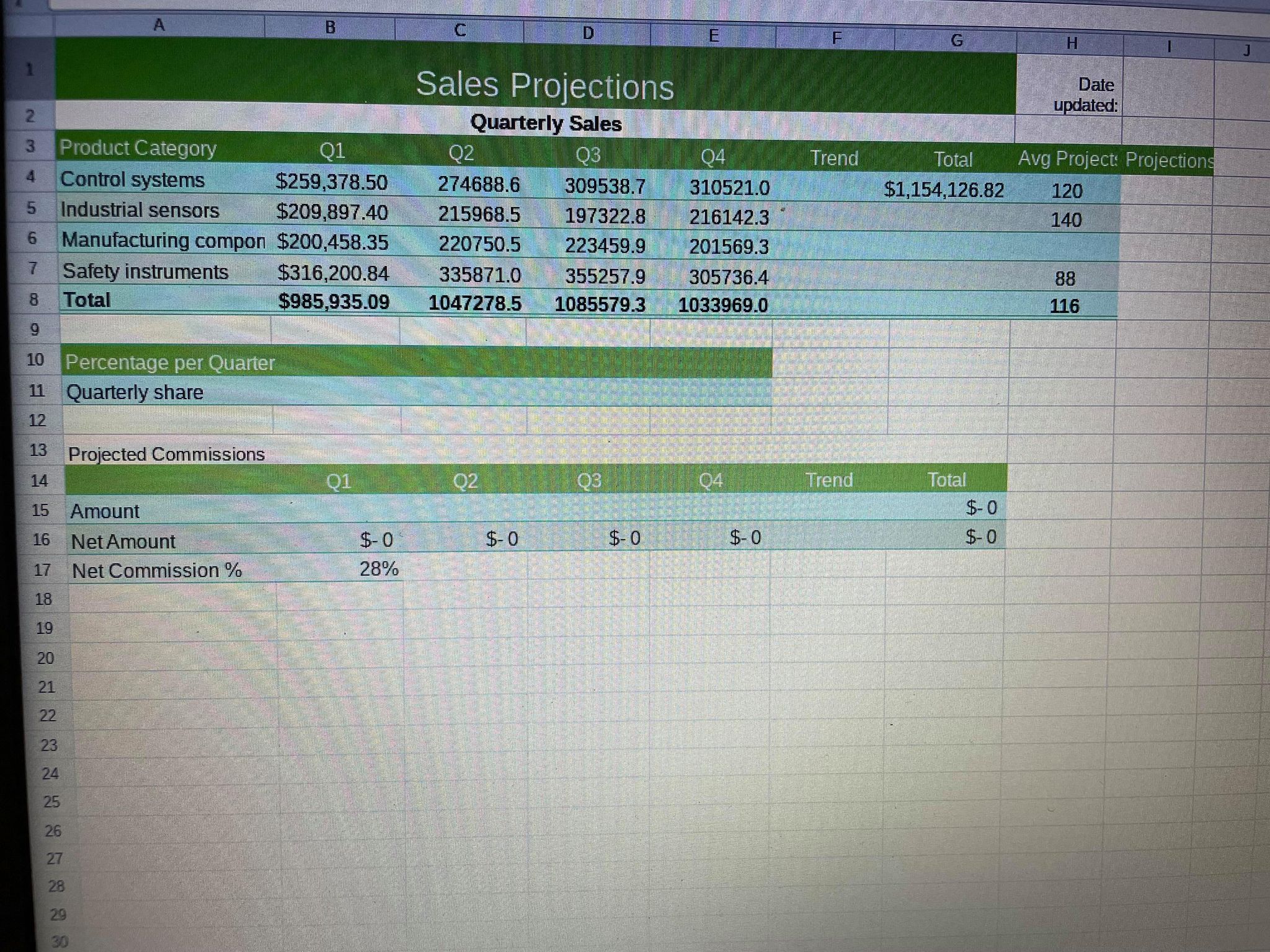
A . A - PROJECT STEPS Janelle Duong is a financial analyst for Avero International, a global company in San Diego, California, that provides automation products to manufacturing businesses. Janelle has been creating sales projections in an Excel workbook, and has asked you to help her complete the worksheet. Go to the Sales Projections worksheet. Middle-align the contents of the merged cell Al. Italicize the contents of cell H1. In cell I1, insert a formula that uses the NOW function to display today's date. Apply the formatting in the merged cell D2 to the merged cell A13. Fill the range C4:E8 with only the formatting from the range B4:BS. In cell F4, insert a Line sparkline based on the data in the range B4:E4. Fill the range F5:F8 without formatting based on the contents of cell F4. Change the color of the sparklines to Dark Blue, Text 2, and then add markers to the sparklines. Copy the formula in cell G4 and paste it in the range G5:G8, pasting only the formula and number formatting. Use Goal Seek to set the average number of projects (cell HS) to the value of 120 by changing the average number of manufacturing component projects (cell H6). Merge and center the range 13:18. Rotate the text down to -90 degrees in the merged cell, and then change the width of column I to 9.25. In cell B11, insert a formula that uses the IFERROR function to divide the total sales for Q1, in cell B8 by the total sales in cell G8 and display "Incorrect" in case of an error. Use an absolute reference to cell G8 in the formula, and then fill the range C11:E11 with the formula in cell B11. CENGAGE Shelly Cashman Excel 2019 | Module 3: End of Module Project 2 In cell B15, enter a formula that uses the IF function and tests whether the total sales for Q1 (cell B8) is greater than or equal to 1000000. If the condition is true, multiply the total sales for Q1 by 0.18 to calculate a commission of 18%, If the condition is false, multiply the total sales for Q1 by 0.10 to calculate a commission of 10%. Fill the range C15:515 with the formula in cell B15 to calculate the commissions for the other three quarters. In cell F15, insert a Column sparkline based on the data in the range 815:515. Fill cell F16B C D E F G H Sales Projections Date updated: NO Quarterly Sales 3 Product Category Q1 OB 04 Trend Total Avg Project: Projections 4 Control systems $259,378.50 274688.6 309538.7 310521.0 $1,154,126.82 120 5 Industrial sensors $209,897.40 215968.5 197322.8 216142.3 140 6 Manufacturing compon $200,458.35 220750.5 223459.9 201569.3 7 Safety instruments $316,200.84 335871.0 355257.9 305736.4 88 8 Total $985,935.09 1047278.5 1085579.3 1033969.0 116 9 10 Percentage per Quarter 11 Quarterly share 12 13 Projected Commissions 14 02 OB 04 Trend Total 15 Amount $-0 16 Net Amount $-0 $-0 $- 0 $-0 $-0 17 Net Commission % 28% 18 19 20A - A . Shelly Cashman Excel 2019 | Module 3: End of Module Project 2 In cell B15, enter a formula that uses the IF function and tests whether the total sales for Q1 {cell BS) is greater than or equal to 1000000. If the condition is true, multiply the total sales for Q1 by 0.18 to calculate a commission of 18%. If the condition is false, multiply the total sales for Q1 by 0.10 to calculate a commission of 10%. Fill the range C15:515 with the formula in cell B15 to calculate the commissions for the other three quarters. In cell F15, insert a Column sparkline based on the data in the range 815:515. Fill cell F16 without formatting based on the contents of cell F15. Display the High Point and the Low Point in the sparklines. Create a clustered column chart based on the range A3 EZ. Resize and reposition the chart so its upper-left corner is in cell A18 and its lower-right corner is in cell G29. Change the chart layout to Quick Layout 9. Enter Projected Sales as the chart title. Enter Sales Amount as the primary vertical axis title. Remove the primary horizontal axis title. Your workbook should look like the Final Figures on the following pages, Save your changes, close the workbook, and then exit Excel. Follow the directions on the SAM website to submit your completed project