please code these questions 3 and 4 on matlab urgent assistance needed with full details

this is all info i have

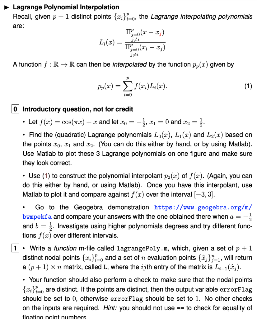
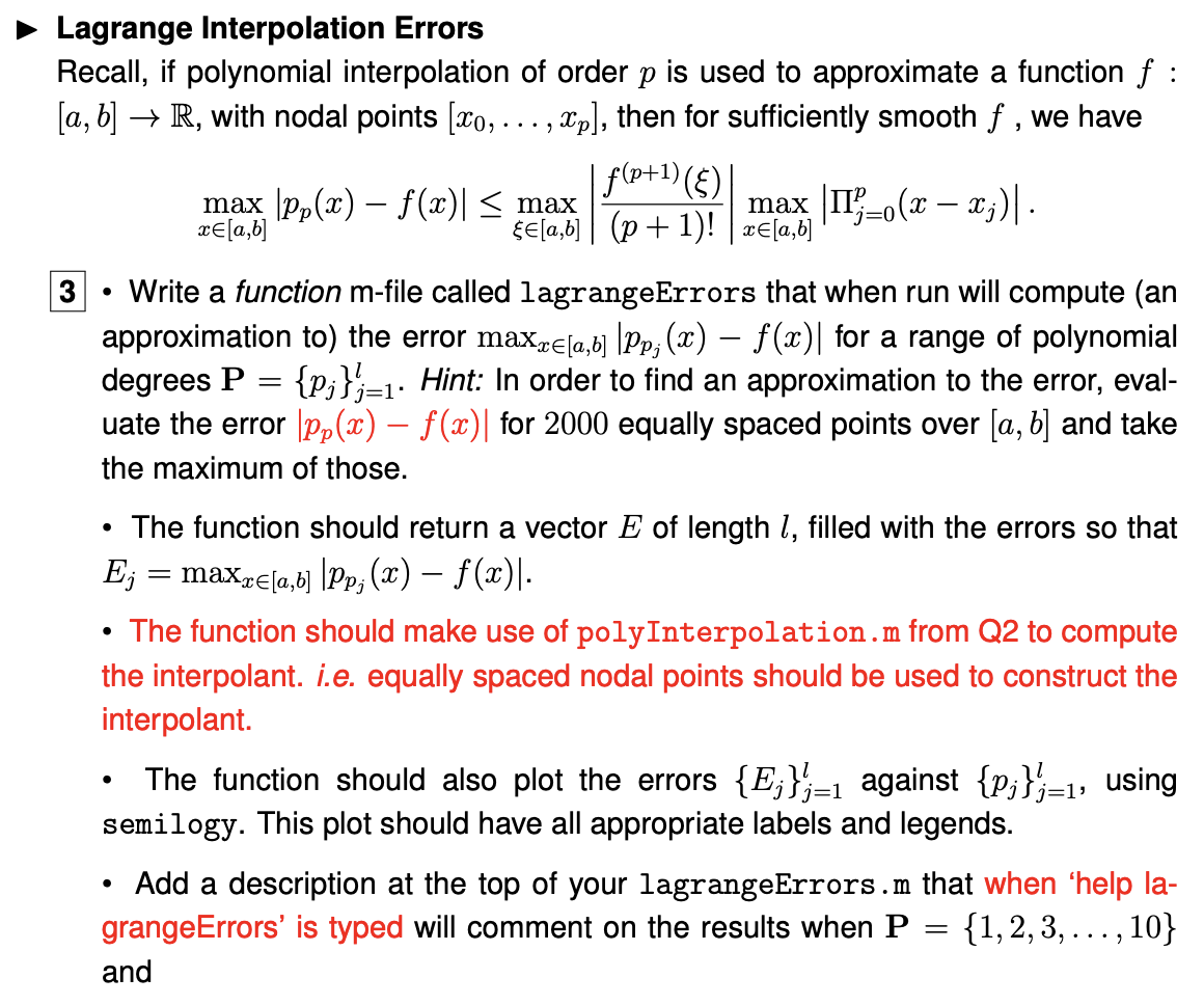
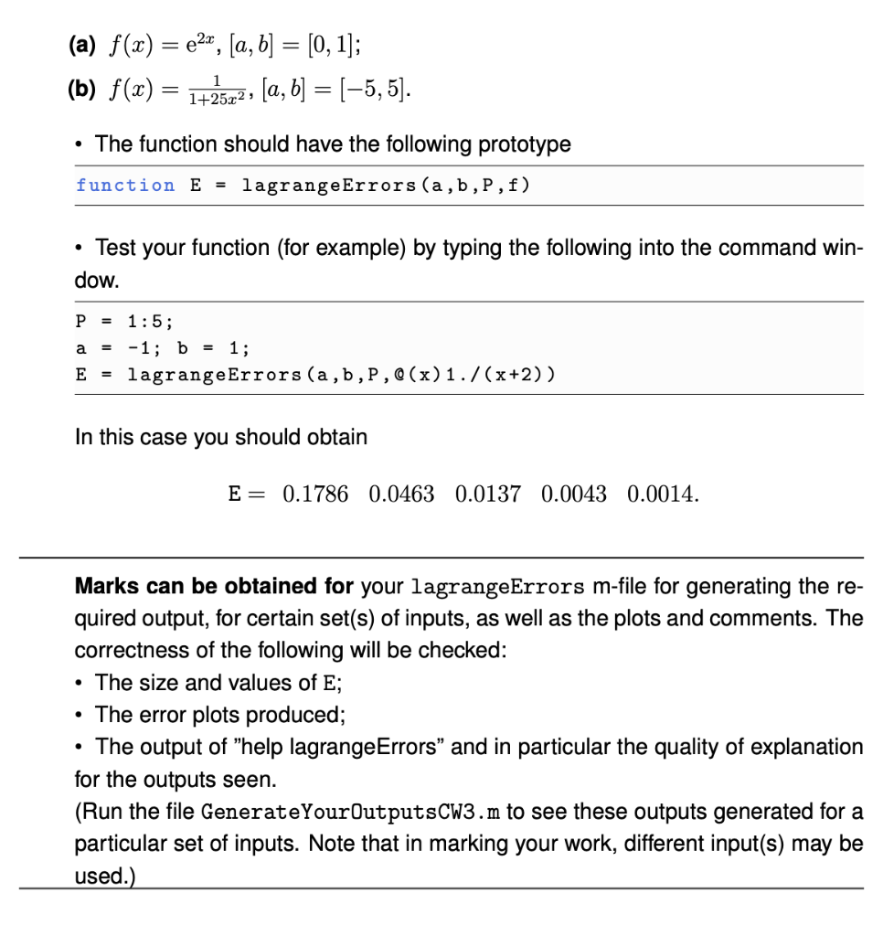
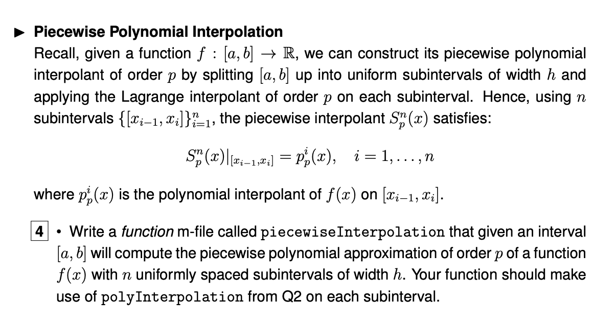
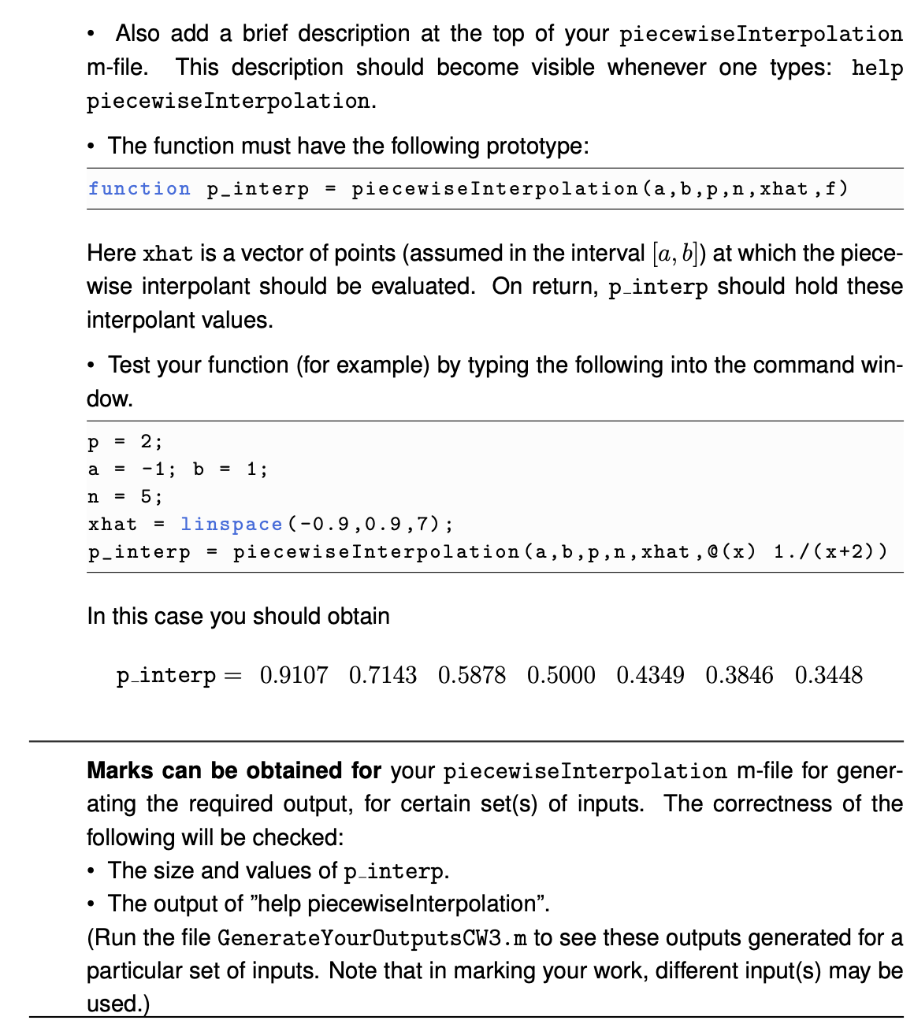
Lagrange Polynomial Interpolation Recall, given p + 1 distinct points {Xi}}=0, the Lagrange interpolating polynomials are: IT';=0 (x X;) iti Li(x) II?0(1; x;) jhi A function f : R + R can then be interpolated by the function pp(x) given by Pp(x) = f(xi)Li(x). /) (1) i=0 Introductory question, not for credit Let f(x) = cos(nx) + x and let xo = = -2, x1 = 0 and X2= Find the (quadratic) Lagrange polynomials Lo(r), L1(x) and L2(x) based on the points zo, 21 and 22. (You can do this either by hand, or by using Matlab). Use Matlab to plot these 3 Lagrange polynomials on one figure and make sure they look correct. Use (1) to construct the polynomial interpolant p2(x) of f(x). (Again, you can do this either by hand, or using Matlab). Once you have this interpolant, use Matlab to plot it and compare against f(x) over the interval (-3, 3). Go to the Geogebra demonstration https://www.geogebra.org/m/ bwmpekfa and compare your answers with the one obtained there when a - and b = 1. Investigate using higher polynomials degrees and try different func- tions f(x) over different intervals. 1 Write a function m-file called lagrangePoly.m, which, given a set of p+1 distinct nodal points {x;}}=o and a set of n evaluation points {@j}}=1, will return a (p+1) x n matrix, called L, where the ijth entry of the matrix is Li1(;). Your function should also perform a check to make sure that the nodal points {{i}}-o are distinct. If the points are distinct, then the output variable errorFlag should be set to 0, otherwise errorFlag should be set to 1. No other checks on the inputs are required. Hint: you should not use == to check for equality of floating point numbers . Lagrange Interpolation Errors Recall, if polynomial interpolation of order p is used to approximate a function f : [a, b] R, with nodal points [20, ..., Xp], then for sufficiently smooth f , we have f(p+1)(E) max Pp() f(x)] = max max (IT)0(x x;)]. Te[a,b] FE[a,b] (P + 1)! | @E[a,b] Write a function m-file called lagrangeErrors that when run will compute (an approximation to) the error max.cE[a,b] \Pp; (2) f(x)] for a range of polynomial degrees P {P;}}=1. Hint: In order to find an approximation to the error, eval- uate the error \pp(x) f(x) for 2000 equally spaced points over [a, b] and take the maximum of those. The function should return a vector E of length 1, filled with the errors so that E; = max,E[a,b] \Pp; (x) f(x)]. The function should make use of polyInterpolation.m from Q2 to compute the interpolant. i.e. equally spaced nodal points should be used to construct the interpolant. The function should also plot the errors {E;}}=1 against {P;}}=1, using semilogy. This plot should have all appropriate labels and legends. Add a description at the top of your lagrangeErrors.m that when 'help la- grangeErrors' is typed will comment on the results when P = {1, 2, 3, ..., 10} and O (a) f(x) = 24, [a, b] = [0, 1]; (b) f(x) = 1+2522, [a, b] = (-5,5). The function should have the following prototype function E lagrange Errors (a,b,P, f) . Test your function (for example) by typing the following into the command win- dow. P = 1:5; = -1; b = 1; E = lagrangeErrors (a, b,P,Q(x)1./(x+2)) a In this case you should obtain E= 0.1786 0.0463 0.0137 0.0043 0.0014. . Marks can be obtained for your lagrangeErrors m-file for generating the re- quired output, for certain set(s) of inputs, as well as the plots and comments. The correctness of the following will be checked: The size and values of E; The error plots produced; The output of "help lagrangeErrors and in particular the quality of explanation for the outputs seen. (Run the file GenerateYourOutputsCW3.m to see these outputs generated for a particular set of inputs. Note that in marking your work, different input(s) may be used.). Piecewise Polynomial Interpolation Recall, given a function f : [a, b] R, we can construct its piecewise polynomial interpolant of order p by splitting [a, b] up into uniform subintervals of width h and applying the Lagrange interpolant of order p on each subinterval. Hence, using n subintervals { [Li1, X]}}=-1, the piecewise interpolant Sy(x) satisfies: Spy (2)|(2:-1,7i] = p(x), i = 1, ...,n where p(x) is the polynomial interpolant of f(x) on (731, Lj]. 4 Write a function m-file called piecewiseInterpolation that given an interval [a, b] will compute the piecewise polynomial approximation of order p of a function f(x) with n uniformly spaced subintervals of width h. Your function should make use of polyInterpolation from Q2 on each subinterval. Also add a brief description at the top of your piecewiseInterpolation m-file. This description should become visible whenever one types: help piecewiseInterpolation. The function must have the following prototype: function p_interp piecewiseInterpolation(a,b,p,n,xhat, f) = Here xhat is a vector of points (assumed in the interval [a, b]) at which the piece- wise interpolant should be evaluated. On return, p_interp should hold these interpolant values. Test your function (for example) by typing the following into the command win- dow. a P = 2; = -1; b = 1; = 5; xhat linspace(-0.9,0.9,7); p-interp piecewiseInterpolation(a,b,p,n,xhat ,@(x) 1./(x+2)) n = In this case you should obtain p-interp = 0.9107 0.7143 0.5878 0.5000 0.4349 0.3846 0.3448 Marks can be obtained for your piecewiseInterpolation m-file for gener- ating the required output, for certain set(s) of inputs. The correctness of the following will be checked: The size and values of p_interp. The output of "help piecewiselnterpolation. (Run the file GenerateYourOutputsCW3.m to see these outputs generated for a particular set of inputs. Note that in marking your work, different input(s) may be used.) . Lagrange Polynomial Interpolation Recall, given p + 1 distinct points {Xi}}=0, the Lagrange interpolating polynomials are: IT';=0 (x X;) iti Li(x) II?0(1; x;) jhi A function f : R + R can then be interpolated by the function pp(x) given by Pp(x) = f(xi)Li(x). /) (1) i=0 Introductory question, not for credit Let f(x) = cos(nx) + x and let xo = = -2, x1 = 0 and X2= Find the (quadratic) Lagrange polynomials Lo(r), L1(x) and L2(x) based on the points zo, 21 and 22. (You can do this either by hand, or by using Matlab). Use Matlab to plot these 3 Lagrange polynomials on one figure and make sure they look correct. Use (1) to construct the polynomial interpolant p2(x) of f(x). (Again, you can do this either by hand, or using Matlab). Once you have this interpolant, use Matlab to plot it and compare against f(x) over the interval (-3, 3). Go to the Geogebra demonstration https://www.geogebra.org/m/ bwmpekfa and compare your answers with the one obtained there when a - and b = 1. Investigate using higher polynomials degrees and try different func- tions f(x) over different intervals. 1 Write a function m-file called lagrangePoly.m, which, given a set of p+1 distinct nodal points {x;}}=o and a set of n evaluation points {@j}}=1, will return a (p+1) x n matrix, called L, where the ijth entry of the matrix is Li1(;). Your function should also perform a check to make sure that the nodal points {{i}}-o are distinct. If the points are distinct, then the output variable errorFlag should be set to 0, otherwise errorFlag should be set to 1. No other checks on the inputs are required. Hint: you should not use == to check for equality of floating point numbers . Lagrange Interpolation Errors Recall, if polynomial interpolation of order p is used to approximate a function f : [a, b] R, with nodal points [20, ..., Xp], then for sufficiently smooth f , we have f(p+1)(E) max Pp() f(x)] = max max (IT)0(x x;)]. Te[a,b] FE[a,b] (P + 1)! | @E[a,b] Write a function m-file called lagrangeErrors that when run will compute (an approximation to) the error max.cE[a,b] \Pp; (2) f(x)] for a range of polynomial degrees P {P;}}=1. Hint: In order to find an approximation to the error, eval- uate the error \pp(x) f(x) for 2000 equally spaced points over [a, b] and take the maximum of those. The function should return a vector E of length 1, filled with the errors so that E; = max,E[a,b] \Pp; (x) f(x)]. The function should make use of polyInterpolation.m from Q2 to compute the interpolant. i.e. equally spaced nodal points should be used to construct the interpolant. The function should also plot the errors {E;}}=1 against {P;}}=1, using semilogy. This plot should have all appropriate labels and legends. Add a description at the top of your lagrangeErrors.m that when 'help la- grangeErrors' is typed will comment on the results when P = {1, 2, 3, ..., 10} and O (a) f(x) = 24, [a, b] = [0, 1]; (b) f(x) = 1+2522, [a, b] = (-5,5). The function should have the following prototype function E lagrange Errors (a,b,P, f) . Test your function (for example) by typing the following into the command win- dow. P = 1:5; = -1; b = 1; E = lagrangeErrors (a, b,P,Q(x)1./(x+2)) a In this case you should obtain E= 0.1786 0.0463 0.0137 0.0043 0.0014. . Marks can be obtained for your lagrangeErrors m-file for generating the re- quired output, for certain set(s) of inputs, as well as the plots and comments. The correctness of the following will be checked: The size and values of E; The error plots produced; The output of "help lagrangeErrors and in particular the quality of explanation for the outputs seen. (Run the file GenerateYourOutputsCW3.m to see these outputs generated for a particular set of inputs. Note that in marking your work, different input(s) may be used.). Piecewise Polynomial Interpolation Recall, given a function f : [a, b] R, we can construct its piecewise polynomial interpolant of order p by splitting [a, b] up into uniform subintervals of width h and applying the Lagrange interpolant of order p on each subinterval. Hence, using n subintervals { [Li1, X]}}=-1, the piecewise interpolant Sy(x) satisfies: Spy (2)|(2:-1,7i] = p(x), i = 1, ...,n where p(x) is the polynomial interpolant of f(x) on (731, Lj]. 4 Write a function m-file called piecewiseInterpolation that given an interval [a, b] will compute the piecewise polynomial approximation of order p of a function f(x) with n uniformly spaced subintervals of width h. Your function should make use of polyInterpolation from Q2 on each subinterval. Also add a brief description at the top of your piecewiseInterpolation m-file. This description should become visible whenever one types: help piecewiseInterpolation. The function must have the following prototype: function p_interp piecewiseInterpolation(a,b,p,n,xhat, f) = Here xhat is a vector of points (assumed in the interval [a, b]) at which the piece- wise interpolant should be evaluated. On return, p_interp should hold these interpolant values. Test your function (for example) by typing the following into the command win- dow. a P = 2; = -1; b = 1; = 5; xhat linspace(-0.9,0.9,7); p-interp piecewiseInterpolation(a,b,p,n,xhat ,@(x) 1./(x+2)) n = In this case you should obtain p-interp = 0.9107 0.7143 0.5878 0.5000 0.4349 0.3846 0.3448 Marks can be obtained for your piecewiseInterpolation m-file for gener- ating the required output, for certain set(s) of inputs. The correctness of the following will be checked: The size and values of p_interp. The output of "help piecewiselnterpolation. (Run the file GenerateYourOutputsCW3.m to see these outputs generated for a particular set of inputs. Note that in marking your work, different input(s) may be used.)