

Question: ****PLEASE DO NOT ANSWER THIS QUESTION UNLESS YOU GIVE THE EXCEL FORMULAS AS THIS IS WHAT THIS QUESTION IS ASKING FOR!!!!!**** The Chestnut Street Company
****PLEASE DO NOT ANSWER THIS QUESTION UNLESS YOU GIVE THE EXCEL FORMULAS AS THIS IS WHAT THIS QUESTION IS ASKING FOR!!!!!****
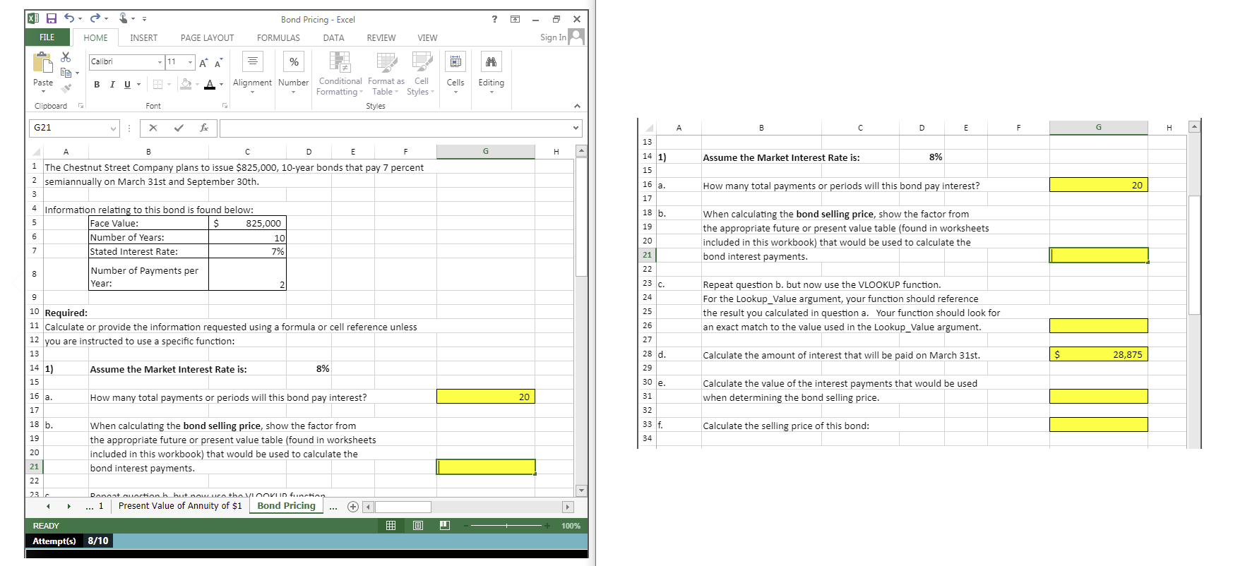
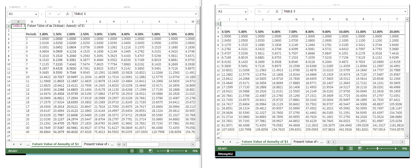
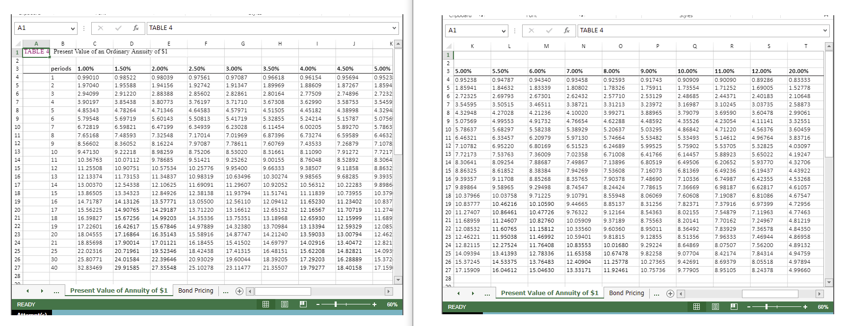
The Chestnut Street Company plans to issue a bond semiannually on March 31st and September 30th.The Controller has asked you to calculate information about the bond assuming two different market interest rates in the Excel Simulation below.The present value factor tables are included in the first four tabs of the Excel Simulation.Use the information included in the Excel Simulation and the Excel functions described below to complete the task.
- Cell Reference:Allows you to refer to data from another cell in the worksheet.From the Excel Simulation below, if in a blank cell, "=C6" was entered, the formula would output the result from cell C6, or 10 in this example.
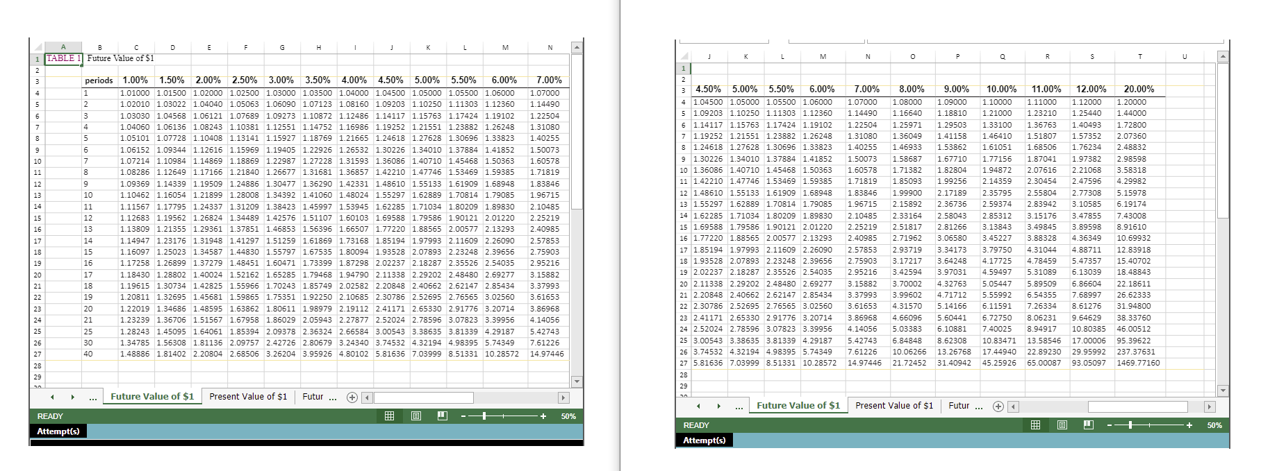
- Multi-Tab Cell Reference:Allows you to refer to data from another cell in a separate tab in the worksheet.When using the multi-tab cell reference, type the equal sign first, then click on the other tab and then click on the cell you want to reference.The syntax of a multi-tab cell reference looks different than a normal cell reference, since it includes the tab name surrounded by apostrophes and also an exclamation point before the cell location.From the Excel Simulation below, if in a blank cell on the Sheet1 tab "='Future Value of $1'!C13" was entered, the formula would output the result from cell C13 in the Future Value of $1 tab, or 1.10462 in this example.
- Basic Math functions:Allows you to use the basic math symbols to perform mathematical functions.You can use the following keys:+ (plus sign to add), - (minus sign to subtract), * (asterisk sign to multiply), and / (forward slash to divide).From the Excel Simulation below, if in a blank cell "=C6+C8" was entered, the formula would add the values from those cells and output the result, or 12 in this example.If using the other math symbols the result would output an appropriate answer for its function.
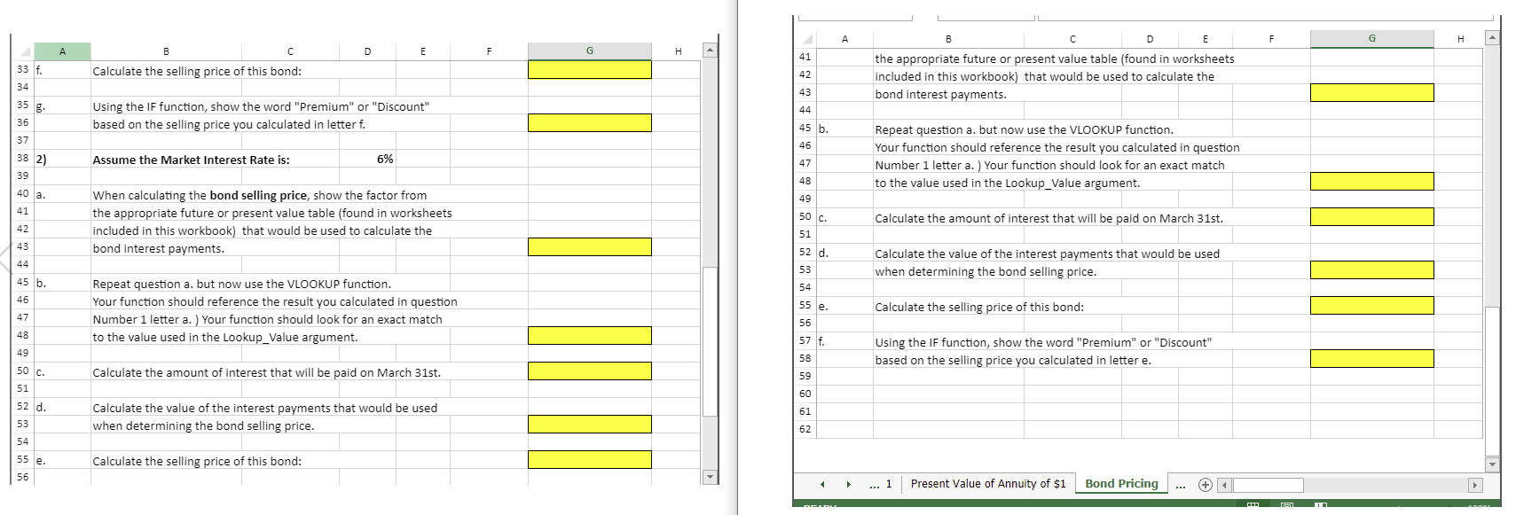
- IF function:Allows you to test a condition and return a specific value is the result is true and different value if the result is false.The syntax of the IF function is "=IF(test_condition,value_if_true,value_if_false)" and specific considerations need to be made when using this function.Thetest_conditionargument is an evaluation of the status of a cell, such as if the value of a cell is greater than, less than, or equal to another number or cell.Thevalue_if_trueandvalue_if_falsearguments will return any specific result for each option, such as another cell reference, a value, or text.Throughout the entire equation, if text is being used in thetest_condition,value_if_true, orvalue_if_falsearguments then the text itself should be entered in quotations so that Excel will recognize the text as a "string of text" instead of another function.From the Excel Simulation below, if in a blank cell "=IF(C6>2,"Long-Term Bond","Short-Term Bond") was entered, the formula would output the result of thevalue_if_truesince thetest_conditionwould be result as true, or in this case the text "Long-Term Bond".Excel processes the IF function by separating it out into separate parts.First thetest_condition- Excel thinks,find cell C6 and determine if the value is greater than 2.Once Excel determines if the result of thattest_conditionis TRUE or FALSE, it will return thevalue_if_trueorvalue_if_false.
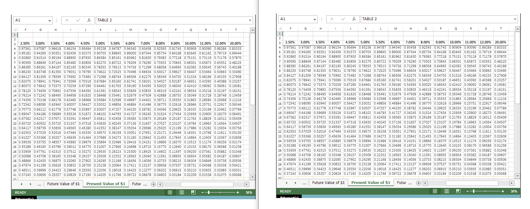
- VLOOKUP Function:Allows you find a value inside of a sorted data table by referencing the column and row labels.The syntax of the VLOOKUP function is "=VLOOKUP(lookup_value,table_array,col_index_num,range_lookup)" and results in a value found from a data table.Thelookup_valueargument is the value to be found in the first column of the table.Thetable_arrayis the cell reference for the data table, usually shown as a range.Thecol_index_numargument is the column number in the data table (table_array) where the matching value should be found.Therange_lookupargument is a logical value of TRUE or FALSE, where TRUE represents the value found in the first column should be a closest match, and FALSE represents the value found in the first column should be an exact match.From the Excel Simulation below, if in a blank cell "=VLOOKUP(C6,'Future Value of $1'!B3:T27,2,FALSE)" was entered, the formula would output the result of 1.10462 in this example.Excel processes the VLOOKUP function by using each argument to find the cross-section of the column and row reference in the data table.In the example, Excel looked at the first column of thetable_arrayon the Future Value of $1 tab cells B3:T27 and found thelookup_value of the Sheet1 cell C6 reference, or 10 periods in this example.That position in the first column is stored in Excel to know what row the final result will be found in.Remember that the first column used is the first column of thetable_arrayand not the first column of the worksheet tab.Then thecol_index_numis used by Excel to determine what column of thetable_arraythe final result is included, or in this case the second column.Excel then finds the cross-section of those two values using the row and column references and outputs the final result from the data table.
Step by Step Solution
There are 3 Steps involved in it
1 Expert Approved Answer
Step: 1 Unlock

Question Has Been Solved by an Expert!
Get step-by-step solutions from verified subject matter experts
Step: 2 Unlock
Step: 3 Unlock