please explain all the formulas

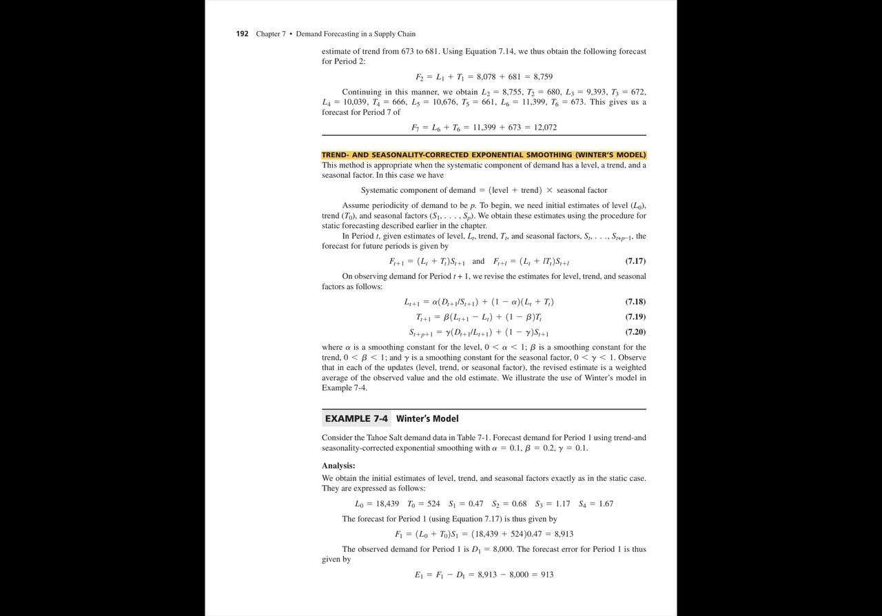
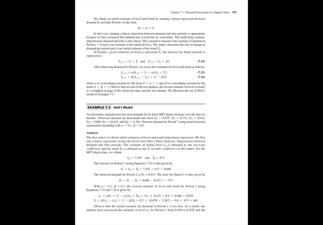
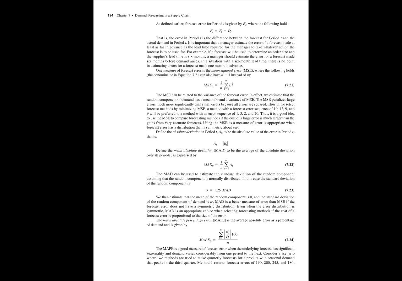
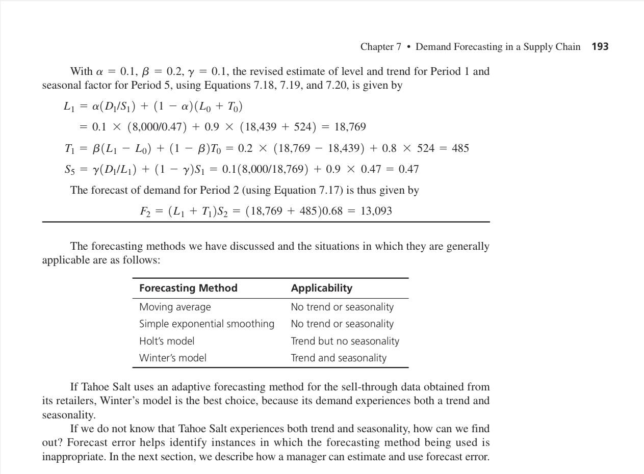
_'_.__. ._ ._: _. _._ The trend-corrected appropnate when demand is assumed to have a level and a trend in the systematic component but no seasonality. In this case, we have Systematic component of demand = level + trend 192 Chapter 7 . Demand Forecasting in a Supply Chain estimate of trend from 673 to 681. Using Equation 7.14, we thus obtain the following forecast for Period 2: F2 = Li + 7) = 8,078 + 681 = 8,759 Continuing in this manner, we obtain Ly = 8.755. 72 = 680, Ly = 9.393. 7, = 672. Ly = 10.039, TA = 666. Ls = 10.676. 75 = 661. Lo = 11.399. 76 = 673. This gives us a forecast for Period 7 of F7 = L6 + To = 11.399 + 673 = 12.072 TREND- AND SEASONALITY-CORRECTED EXPONENTIAL SMOOTHING (WINTER'S MODEL) This method is appropriate when the systematic component of demand has a level, a trend, and a seasonal factor. In this case we have Systematic component of demand = (level + trend) X seasonal factor Assume periodicity of demand to be p. To begin, we need initial estimates of level (Lo). trend (To), and seasonal factors ($1, . .. . S,). We obtain these estimates using the procedure for static forecasting described earlier in the chapter. In Period t. given estimates of level, L, trend, 7,, and seasonal factors. S,. . . .. Step-1. the forecast for future periods is given by Fi+1 = (L, + 7,)S,+1 and F,41 = (L, + IT;)S,41 (7.17) On observing demand for Period f + 1, we revise the estimates for level, trend, and seasonal factors as follows: LI41 = a( D,+1/5,+1) + (1 - @)(L, + 1,) (7.18) ,+1 = B(L,+1 - L,) + (1 - B)T, 7.19) Sip+1 = Y(D,+1/L,+1) + (1 - >)$,41 (7.20) where a is a smoothing constant for the level. 0 + 6). This may happen because the forecasting method is awed or the underlying demand pattern has shifted. One instance in which a large negative TS will result occurs when demand has a growth trend and the manager is using a forecasting method such as moving average. Because trend is not included, the average of historical demand is always lower than future demand. The negative TS detects that the forecasting method consistently underestimates demand and alerts the manager. The tracking signal may also get large when demand has suddenly dropped (as it did for many industries in 2009) or increased by a signicant amount making historical data less relevant. If demand has suddenly dropped, it makes sense to increase the weight on current data relative to older data when making forecasts. McClain (1981) recommends the \"declining alpha\" method when using exponential smoothing where the smoothing constant starts large (to give greater weight to recent data) but then decreases over time. If we are aiming for a long-term smoothing constant of 0: = 1 p, a declining alpha approach would be to start with 0:0 : 1 and reset the smoothing constant as follows: \":71 1 7 P a! p+aril1_Pr In the long term, the smoothing constant will converge to a : 1 p with the forecasts becoming more stable over time