Question: please follow the instructions provided on the excel spreadsheet. Make sure to include the cell number and formulas required to yield the answers to part

please follow the instructions provided on the excel spreadsheet. Make sure to include the cell number and formulas required to yield the answers to part one and two.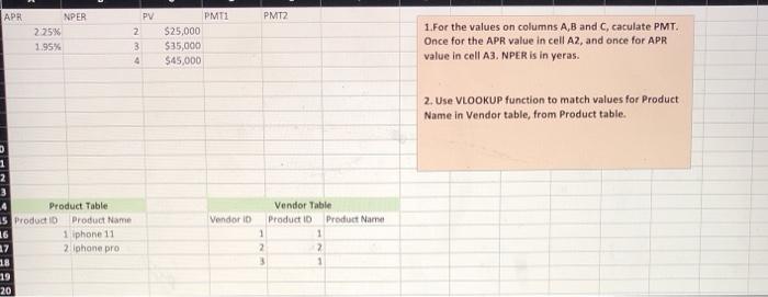

APR PMT2 NPER 225% 1.95% PV 2 3 4 PMT1 $25,000 $35,000 $45,000 1.For the values on columns A,B and C, caculate PMT. Once for the APR value in cell A2, and once for APR value in cell A3, NPER is in yeras. 2. Use VLOOKUP function to match values for Product Name in Vendor table, from Product table. Vendor ID 1 2 3 Product Table 5 Product ID Product Name 16 1 iphone 11 27 2 iphone pro 18 19 20 Vendor Table Product 10 Product Name 1 1 2 2 3 1

Step by Step Solution

There are 3 Steps involved in it

1 Expert Approved Answer

Step: 1 Unlock blur-text-image

Question Has Been Solved by an Expert!

Get step-by-step solutions from verified subject matter experts

Step: 2 Unlock

Step: 3 Unlock

Students Have Also Explored These Related Databases Questions!

The Business This practice set is designed to be five parts. In the first part, the student will complete the journal entries by writing the journal entries for Ivan's Instruments in the template...

Part One Instructions Record the September 2023 transactions, journal entries, in an Excel Spreadsheet. An example of an Excel spreadsheet follows the transactions below. No explanation is required...

PRACTICE NUMBER 5 I NEED HELP below. Chart of Accounts Current Assets 10000 Cash ma 11000 Accounts Receivable 12000 Inventory-Orange Roller Blades 12100 Inventory - Black Roller Blades 13100 Office...

Case for Digital Assets Semester: 5 rln 2023 Name: I II Total Points Possible: 20 FinalScore- Final Percentage: On each tab of this spreadsheet you will find instructions to help you complete the...

Hi this is for my accounting class, if someone can help me it would be very helpful, thanks! Part One Instructions Record the January 2021 transactions, journal entries, in an Excel Spreadsheet. An...

HI ,THE INSTRUCTIONS ARE INCLUDED IN THE PICTURE .THANK YOU . Current Assets 10000 Cash 11000 Accounts Receivable 12000 Inventory - 26" Bikes 12050 Inventory - 20" Bikes 13000 Office Supplies 13050...

Help please, I need the Journal Entries for each transaction C ACCOUNTING Part One Instructions Record the September 2021 transactions, Journal entries, in an Excel Spreadsheet. An example of an...

Option #1: Individual Tax ReturnsCase 1 Because it is important for accountants to demonstrate the filing requirements for individual tax returns, for this final project you will be completing an...

FIN310 Graded Project: Corporate Finance Your project must be submitted as an Excel document. Your project will be individually graded by your instructor and, therefore, will take up to a few weeks...

Graded Project Ice Cream Systems CONTENTS PROJECT GOAL 2 PROJECT INFORMATION 3 PROJECT INSTRUCTIONS 15 SUBMITTING YOUR PROJECT 26 GRADING CRITERIA 26 PLAGIARISM\t27 PENN FOSTER, INC. 2017 ICE CREAM...

XCO pays $500,000 for a 30% interest in ZCO. XCO uses the equity method to account for this investment. At the end of the first year, ZCO has total earnings of $120,000 and has made total...

On January 1, 20Y1 Caitlin Corporation issued $10 million in 10-year bonds. The bonds pay 7% interest annually on December 31. At issuance, the market rate of interest for bonds of comparable risk...

Arturn to cuestlo Required information [ The following information applies to the questions displayed below ] Carrie DLake, Reed A . Green, and Doug A . Divot share a passion for golf and decide to...

Seved Help 14 Wisconsin Snowmobile Corp. is considering a switch to level production Cost efficiencies would occur under level production, and aftertax costs would decline by $31,500, but inventory...

3. Are our bosses always right? If not, what should we do?

2. What, according to Sergey, was strange at this meeting?

1. Opportunities for face-to-face contact will be diminished, and information from nonverbal cues will be reduced. Consequently, opportunities for random spontaneous information sharing will be...