PLEASE HELP EXCEL, DO NOT KNOW HOW TO WORK IT AT ALL, PLEASE INCLUDE DIRECTIONS IF YOU CAN.

I HAVE PROVIDED A LINK TO THE SPREADSHEET, LET ME KNOW IF IT DOES NOT WORK, DO TRY TO COPY AND PASTE IT.

https://1drv.ms/x/s!Aul4ImEgkmHEgx1k5CE3xUr12ezS

BELOW ARE SCREENSHOTS OF THE RESPECTIVE EXCEL SHEETS SHOULD THE LINK NOT WORK AS WELL AS THE DIRECTIONS! PLEASE HELP I POSTED THIS EARLIER BUT THE ANSWER WAS JUST SCREENSHOTS OF THE FINISHED PRODUCT AND I DO NOT KNOW HOW IT WAS DONE!

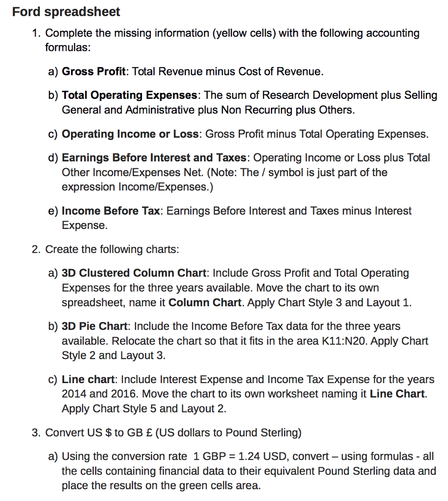
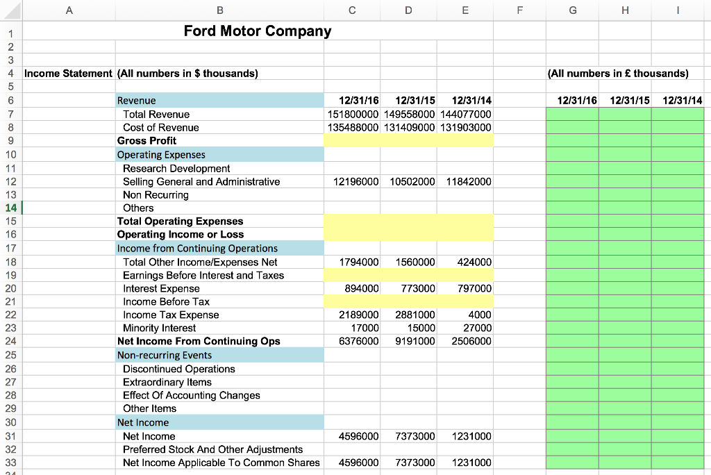
Ford spreadsheet 1. Complete the missing information (yellow cells) with the following accounting formulas a) Gross Profit: Total Revenue minus Cost of Revenue b) Total operating Expenses: The sum of Research Development plus selling General and Administrative plus Non Recurring plus Others c) operating income or Loss: Gross Profit minus Total Operating Expenses. d) Earnings Before Interest and Taxes: Operating Income or Loss plus Total Other Income/Expenses Net. (Note: The symbol is just part of the expression Income/Expenses.) e) Income Before Tax: Earnings Before Interest and Taxes minus Interest Expense 2. Create the following charts: a) 3D Clustered Column Chart: Include Gross Profit and Total Operating Expenses for the three years available. Move the chart to its own spreadsheet, name it Column Chart. Apply Chart Style 3 and Layout 1. b) 3D Pie Chart: Include the Income Before Tax data for the three years available. Relocate the chart so that it fits in the area K11:N20. Apply Chart Style 2 and Layout 3 c) Line chart: Include Interest Expense and Income Tax Expense for the years 2014 and 2016. Move the chart to its own worksheet naming it Line Chart. Apply Chart Style 5 and Layout 2. 3. Convert US to GB E (US dollars to Pound Sterling) a) Using the conversion rate 1 GBP -1.24 USD, convert -using formulas all the cells containing financial data to their equivalent Pound Sterling data and place the results on the green cells area. Ford spreadsheet 1. Complete the missing information (yellow cells) with the following accounting formulas a) Gross Profit: Total Revenue minus Cost of Revenue b) Total operating Expenses: The sum of Research Development plus selling General and Administrative plus Non Recurring plus Others c) operating income or Loss: Gross Profit minus Total Operating Expenses. d) Earnings Before Interest and Taxes: Operating Income or Loss plus Total Other Income/Expenses Net. (Note: The symbol is just part of the expression Income/Expenses.) e) Income Before Tax: Earnings Before Interest and Taxes minus Interest Expense 2. Create the following charts: a) 3D Clustered Column Chart: Include Gross Profit and Total Operating Expenses for the three years available. Move the chart to its own spreadsheet, name it Column Chart. Apply Chart Style 3 and Layout 1. b) 3D Pie Chart: Include the Income Before Tax data for the three years available. Relocate the chart so that it fits in the area K11:N20. Apply Chart Style 2 and Layout 3 c) Line chart: Include Interest Expense and Income Tax Expense for the years 2014 and 2016. Move the chart to its own worksheet naming it Line Chart. Apply Chart Style 5 and Layout 2. 3. Convert US to GB E (US dollars to Pound Sterling) a) Using the conversion rate 1 GBP -1.24 USD, convert -using formulas all the cells containing financial data to their equivalent Pound Sterling data and place the results on the green cells area