Please help fill up the excel below!!

Suppose a beverage company is considering adding a new product line. Currently the company sells apple juice and they are considering selling a fruit drink. The fruit drink will have a selling price of $1.00 per jar. The plant has excess capacity in a fully depreciated building to process the fruit drink. The fruit drink will be discontinued in four years. The new equipment is depreciated to zero using straight line depreciation. The new fruit drink requires an increase in working capital of $25,000 and $5,000 of this increase is offset with accounts payable. Projected sales are 150,000 jars of fruit drink the first year, with a 20 percent growth for the following years. Variable costs are 55% of total revenues and fixed costs are $10,000 each year. The new equipment costs $195,000 and has a salvage value of $25,000. Bond Information The corporate tax rate is 35 percent and the company currently has 1,000,000 shares of stock outstanding at a current price of $15. The company also has 50,000 bonds outstanding, with a current price of $985. The bonds pay interest semi-annually at the coupon rate is 6%. The bonds have a par value of $1,000 and will mature in twenty years. Equity Information Even though the company has stock outstanding it is not publicly traded. Therefore, there is no publicly available financial information. However, management believes that given the industry they are in the most reasonable comparable publicly traded company is National Beverage Company (ticker symble is FIZZ). In addition, management believes the S&P 500 is a reasonable proxy for the market portfolio. Therefore, the cost of equity is calculated using the beta from FIZZ and the market risk premium based on the S&P 500 annual expected rate of return. (The best estimate for the expected return on the market is to look at long run historical averages of the stock market. I provided you the historical long run average in Module 6 under page Historical Asset Averages. Next go to US Treasury Yield website to obtain current 3 month T-bill rate.) WACC is then calculated using the CAPM and beta estimate as discussed for FIZZ since it is in the same industry. Clearly show all your calculations and sources for all parameter estimates used in the WACC.

1. Calculate the WACC for the company.

2. Create a partial income statement incremental cash flows from this project in the Blank Template worksheet using the tab below.

3. Enter formulas to calculate the NPV by finding the PV of the cash flows over the next four years. (You can either use the EXCEL formula PV() or use mathmatical formula for PV of a lump sum.)

4. Set up the EXCEL worksheet so that you are able to change the parameters in E3 to E12. Run three cases best, most likely, and worst case where the growth rate is 30%, 20%, and 5%, respectfully.

5. Create a NPV profile for the most likely case scenario. (See NPV Calculation tab below.)

6. State whether the company should accept or reject the project for each case scenario.

7. Summarize your recommendation on a one-page pdf or doc file with the following: a. NPV for each case b. NPV profile graph for most likely case c. Very brief (two or three sentence at most) recommendation of accepting or rejecting project. d. Your brief recommendation should include a note stating which parameter estimates you are most uncertain of.

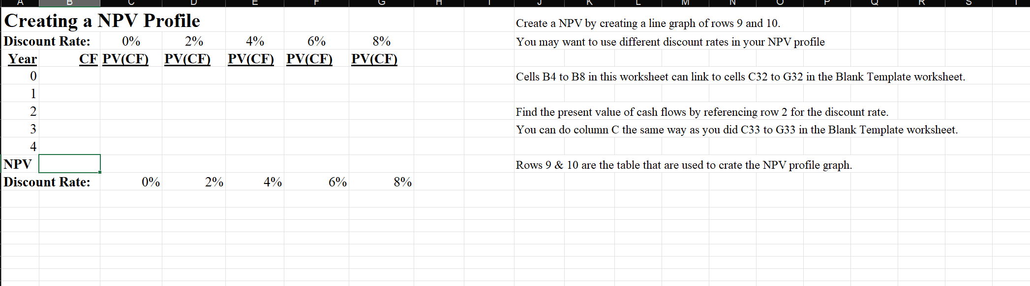
Create a NPV by creating a line graph of rows 9 and 10 . You may want to use different discount rates in your NPV profile Cells B4 to B8 in this worksheet can link to cells C32 to G32 in the Blank Template worksheet. Find the present value of cash flows by referencing row 2 for the discount rate. You can do column C the same way as you did C33 to G33 in the Blank Template worksheet. Rows 9&10 are the table that are used to crate the NPV profile graph. Create a NPV by creating a line graph of rows 9 and 10 . You may want to use different discount rates in your NPV profile Cells B4 to B8 in this worksheet can link to cells C32 to G32 in the Blank Template worksheet. Find the present value of cash flows by referencing row 2 for the discount rate. You can do column C the same way as you did C33 to G33 in the Blank Template worksheet. Rows 9&10 are the table that are used to crate the NPV profile graph